Preface: Why Context Length Is a Hardware Problem Wearing a Software Costume
The promise of long context is seductive: feed a model an entire codebase, a legal corpus, or a year of financial reports and ask it to reason across all of it. The reality is that extending a transformer to 1 million tokens is not primarily a research problem. It is a systems engineering problem with three distinct walls — each physically grounded, each demanding a different class of solution. An engineer who cannot quantify all three at target context length before writing a line of code will hit each wall in production, serially, and expensively.
This article treats those three walls as first principles, then builds the engineering stack on top of them.
Part 1: The Three Walls of Long Context — Quantified at 1M Tokens
Wall 1: Quadratic Attention Compute
Standard scaled-dot-product attention computes, for each of H heads:
S = QKᵀ / √d where Q, K, V ∈ ℝ^{N×d}P = softmax(S)O = PVThe core operation — QKᵀ — is O(N² · d). For N = 1,000,000 tokens, d = 128, and H = 32 heads in FP16:
FLOPs ≈ 2 × N² × d × H = 2 × 10¹² × 128 × 32 ≈ 8.19 × 10¹⁵ FLOPsAt H100 peak FP16 throughput of ~989 TFLOPS and a realistic 40% MFU:
T_compute ≈ 8.19 × 10¹⁵ / (989 × 10¹² × 0.4) ≈ 20.7 seconds per forward pass, per layerAn 80-layer model executes this 80 times. The single forward pass of attention at 1M tokens costs on the order of 1,600 GPU-seconds of compute at realistic utilization. This is not a theoretical concern. It is a scheduling crisis — before you have generated a single output token.
Wall 2: Linear KV Cache Memory
During autoregressive decoding, every previously processed token’s key and value projections must be retained in HBM for each new token’s attention calculation. The KV cache grows linearly with sequence length:
KV cache size = 2 × N × d × H × num_layers × sizeof(dtype)For Llama-3-70B (80 layers, 8 GQA groups, d=128) in BF16 at N = 1,000,000:
= 2 × 1,000,000 × 128 × 8 × 80 × 2 bytes= 327.68 GBA single H100 carries 80 GB of HBM. An H200 carries 141 GB. Neither fits the KV cache of a 1M-context 70B model even before loading the model weights (which themselves consume ~140 GB in BF16). This is not a memory pressure problem; it is a memory impossibility problem on any single device in commercial production today.
The B200 at 192 GB HBM3e changes the arithmetic but does not resolve it: a 70B model at 1M context still requires roughly 4× the B200’s HBM budget for KV cache alone.
Wall 3: Positional Encoding Extrapolation
Transformers trained with fixed positional embeddings — sinusoidal (Vaswani et al., 2017) or learned — degrade catastrophically beyond their training context window. The attention score between query at position i and key at position j is modulated by the angle between their rotary position encoding vectors; at positions far beyond training length, those angles enter uncharacterized regions of the embedding space, producing incoherent attention distributions.
Rotary Position Embeddings (RoPE, Su et al., 2021) fare better but are not immune. RoPE encodes relative position as a rotation matrix in head-dimension space; beyond training length, the high-frequency dimensions cycle through angles that were never trained, causing effective perplexity spikes. At 1M tokens with a model trained at 4K, every token beyond position 4,000 is structurally outside the model’s learned distribution.
This is not fixable by fine-tuning alone. It requires either positional interpolation (scaling the RoPE base frequency — covered in the RoPE scaling section below) or a fundamentally different positional scheme.
Summary at 1M tokens:
| Wall | Magnitude | Production Implication |
|---|---|---|
| Quadratic compute | ~20s per layer per forward pass on H100 | Prefill latency makes 1M naive attention unusable |
| Linear KV cache | 327+ GB for 70B model | Does not fit any single commercial GPU |
| Positional extrapolation | Complete distribution shift past training window | Accuracy collapses without architectural mitigation |
None of these walls yield to more compute alone. Each demands a structural rethink.
Part 2: Sliding Window Attention — Containing the Quadratic
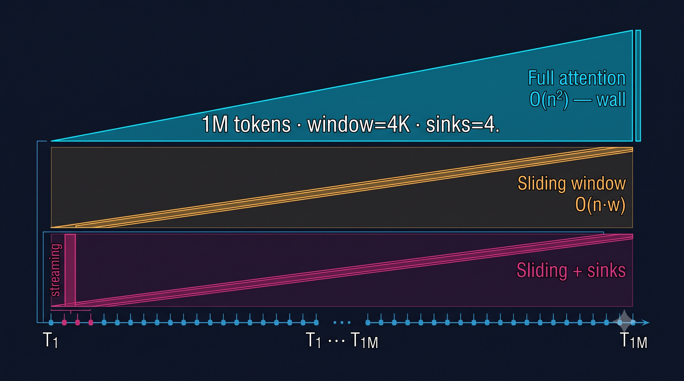
The first engineering response to the quadratic wall is local attention. The Longformer (Beltagy et al., 2020, arXiv:2004.05150) introduced the sliding window pattern into modern NLP: each token attends to the w tokens immediately preceding and following it, rather than all N tokens in the sequence. Compute drops from O(N²) to O(N × w).
At N = 1,000,000 and w = 4,096:
FLOPs_sliding ≈ 2 × N × w × d × H = 2 × 10⁶ × 4,096 × 128 × 32 ≈ 33.6 × 10¹² FLOPs per layerversus the naive 8.19 × 10¹⁵. That is a ~244× reduction in attention FLOPs per layer. Prefill becomes tractable.
Mistral 7B (Jiang et al., 2023) operationalized this at production scale, using a sliding window of w = 4,096 across most attention heads. Crucially, Mistral demonstrated that a relatively narrow local window is empirically sufficient for a wide range of tasks — the model’s residual stream accumulates global context across layers even when each layer’s attention is local. A token at position 100,000 attends to positions 96,000–104,000 directly, but has already accumulated information from all prior positions through the stacked residual path.
The KV cache memory improvement is symmetrical: only the w most recent keys and values need to be retained per layer during decoding, reducing KV cache from linear-in-N to linear-in-w. For a 70B model at w = 4,096:
KV cache_sliding = 2 × 4,096 × 128 × 8 × 80 × 2 bytes ≈ 1.34 GBThis fits comfortably in a single H100. The cost is a hard horizon: tokens outside the window are invisible to any given layer’s attention, and information from the distant past can only propagate forward through the residual accumulation path. For tasks that require precise verbatim recall of early tokens — a specific number or clause from page one of a 10,000-page document — local attention fails without additional machinery.
Part 3: The Attention Sink — Why Throwing Away the Past Fails
Local attention’s memory benefit is real, but naive eviction of old tokens from the KV cache destroys model stability. Xiao et al. (2023, arXiv:2309.17453) — the StreamingLLM paper — identified why through a deceptively simple observation: attention weights are not uniformly distributed across the visible window.
When measuring where attention mass concentrates in a transformer during long-sequence decoding, the first few tokens in the sequence (often positions 0 through 3) receive disproportionately large attention weights — sometimes absorbing 20–40% of the total softmax mass — regardless of their semantic content. This holds even when those initial tokens are padding, BOS markers, or otherwise semantically empty.
The Softmax Sink Mechanism
Understanding why requires thinking about what softmax must do. In standard attention:
P_i = softmax(Q_i Kᵀ / √d)The softmax output must sum to 1.0 across all attended positions. When a query Q_i has no strong alignment with any key — which happens frequently in long contexts where most tokens are semantically distant from the current query — the softmax distribution still must place its probability mass somewhere. It cannot distribute it evenly across all positions when the dot products are highly negative for most positions (the magnitude of QK dot products tends to grow with position due to training distribution shifts).
The solution the model learns is to use a small set of “sink” tokens — positions that accumulate the otherwise-unassignable probability mass. The first token in a sequence is a natural sink candidate: it is always present, always in the window, and its key vectors are shaped by training to absorb surplus attention weight. The model learns to use initial tokens as a softmax normalization sponge.
Empirically, removing the sink tokens and retaining only recent window tokens causes catastrophic instability: the model’s softmax distributions become unnormalized in practice (the available keys cannot absorb the required mass), leading to attention outputs that explode or collapse, and perplexity that degrades even for the tokens nominally within the local window.
The fix is architectural and elegant: retain the first k tokens (typically 4–8) as permanent sinks regardless of the sliding window eviction policy. These tokens never leave the KV cache. All other tokens are evicted on a FIFO basis as the window advances.
Part 4: Combining the Two — Bounded-Memory Streaming Attention
Sliding window + sink tokens yields a KV cache that is both bounded in size and stable in behavior across arbitrarily long sequences. The memory profile becomes:
KV cache_stream = 2 × (k_sink + w) × d × H_GQA × L × sizeof(dtype)For k_sink = 4, w = 4,096, the 70B model specification used above:
≈ 2 × 4,100 × 128 × 8 × 80 × 2 ≈ 1.34 GBThis is O(1) in sequence length — the KV cache does not grow as the sequence extends. The practical consequence is that a model can, in principle, run indefinitely long inference sessions on a single GPU without memory growth, provided the task does not require cross-document recall of arbitrary tokens from arbitrarily far back.
StreamingLLM validated this on Llama-2 models extended to 4 million tokens on a single consumer GPU. The perplexity profile over extended generation remained stable — it did not drift upward — as long as sink tokens were preserved. The model was not comprehending the full 4M-token context (it could not attend backward beyond w), but it was not breaking either. For streaming applications — chatbots maintaining long conversations, code assistants working through a long editing session — this regime is production-viable today.
The engineering implementation is a ring buffer over the KV cache, where positions [k_sink, k_sink + w] rotate on a circular basis, while positions [0, k_sink] are pinned. A single pointer tracks the current oldest evictable position. Implementation overhead is negligible.
Part 5: Hybrid Architectures — When You Need Both Local and Global
For applications that do require global context — answering questions about arbitrarily distant tokens, not just recent ones — neither pure sliding window nor streaming attention suffices. The production answer is hybrid architectures that interleave locally-attending and globally-attending layers.
Gemini 1.5 (Reid et al., 2024) achieves 1M-token context through a mixture-of-expert architecture that augments sparse attention with efficient cross-document retrieval mechanisms, effectively embedding a retrieval system within the transformer’s attention layers rather than as an external component. The architecture enables “needle-in-a-haystack” retrieval across the full 1M-token window — finding a specific fact planted anywhere in the context — a capability that pure sliding-window attention structurally cannot deliver.
Jamba (Lieber et al., 2024, arXiv:2403.19887) represents a categorically different hybrid approach: interleaving Mamba (a state-space model) layers with standard transformer attention layers. Mamba processes sequence information through a learned hidden state that compresses history into a fixed-size representation — a constant-memory operation regardless of sequence length. The hybrid 1:7 ratio (one attention layer per seven Mamba layers) preserves the long-range associative recall capacity of full attention for key positions while letting Mamba handle the bulk of sequential processing at O(N) cost.
The tradeoff is precisely characterized: Mamba’s compressed state is lossy. It cannot retrieve verbatim content from arbitrary positions the way attention can. The interleaved design says: use attention sparingly for the positions where exact recall matters, and let Mamba carry the representational load elsewhere. On practical benchmarks — long-document QA, multi-step reasoning — Jamba matched or exceeded pure transformer baselines at a fraction of the inference compute.
Mistral’s interleaved sliding/full layers take a third approach: most layers use the local sliding window (w = 4,096), while a subset of layers use full attention. This provides a regular global attention “spine” — every few layers, the residual stream is updated with full-context attention — without paying the full quadratic cost at every layer. The full-attention layers are the expensive ones and should be scheduled with care: placing them at the middle and top of the network, where representations are most semantically abstracted, costs the least perplexity per FLOP.
Part 6: RoPE Scaling for Length Extension
No architectural modification to attention patterns solves the positional encoding extrapolation problem. A model trained at 4K must have its positional encoding scheme explicitly extended to handle longer sequences.
The standard approach for RoPE-based models is base frequency scaling (introduced in the “Extending Context Window of Large Language Models via Positional Interpolation” work, Chen et al., 2023). RoPE encodes position m in dimension pair (2i, 2i+1) as a rotation by angle m × θ_i, where:
θ_i = base^{-2i/d}The original RoPE uses base = 10,000. To extend context without retraining, the base is scaled upward:
base_new = base × (L_new / L_train)^{d/(d-2)}For extending from 4K to 128K, this implies base_new ≈ 500,000. The higher base reduces the rotation speed of high-frequency dimensions, stretching the positional embedding space across the longer range. Llama-3’s 128K context extension uses base = 500,000; Code Llama’s context extension (to 100K) used a similar scaling.
The critical insight is that base scaling alone is insufficient for large extension ratios without continued pretraining (or at minimum, fine-tuning) on long-context examples. The model has never seen the new position angles during pretraining; scaling the base changes the geometry but does not train the model to use it. Long-context fine-tuning — even on a fraction of the pretraining data volume — is necessary to achieve stable accuracy at extended lengths.
YaRN (Peng et al., 2023) extends the interpolation approach by applying different scaling factors to different frequency bands of RoPE: high-frequency dimensions (short-range positional signals) are left unscaled or lightly scaled, while low-frequency dimensions (long-range signals) receive aggressive interpolation. This preserves short-range positional fidelity while extending long-range coverage, yielding better perplexity than uniform base scaling at the same extension ratio.
Part 7: The Production Reality — When RAG Beats Native Long Context
The architectural machinery above exists to extend the context window. The engineering question is whether a longer context window is actually the right solution for a given production use case.
Consider a document retrieval system where the corpus is 10 million tokens — orders of magnitude beyond any single context window. The comparison is:
Option A: Native long-context model (128K tokens). Feed the 128K most relevant tokens. Option B: RAG pipeline. Retrieve the 8K most semantically relevant passages, feed to a standard model.
Option B is almost always more economical. Retrieval-augmented generation concentrates compute on the tokens that matter; a 1M-token context window is largely dark (unattended) for most queries. The cost difference at inference is substantial: at 1M tokens, a single prefill pass for a 70B model costs on the order of $2–5 in GPU-hours at current cloud rates. A well-tuned RAG retrieval step costs cents.
The quality comparison is more nuanced. Dense retrieval fails for:
- Queries requiring reasoning over interactions between documents (A says X, B says Y, what are the implications?)
- Tasks where the absence of a signal across many documents is the answer
- Code understanding where the relevant context is dispersed non-contiguously across a large repo
In all three cases, retrieval fundamentally cannot pre-select the right context because relevance is not a property of individual passages — it is a property of their combination.
The honest production calculus is this: RAG is cheaper and often better for retrieval tasks. Native long context is irreplaceable for reasoning tasks. Conflating the two categories is the most expensive mistake in long-context system design.
Part 8: Where Native Long Context Is Truly Irreplaceable
There are three task families where no retrieval scheme substitutes for native context:
1. Code Understanding and Repository-Scale Reasoning
A function’s behavior depends on its callers, its callees, the type definitions it uses, the configuration it reads, and the tests that constrain it. These dependencies are non-local; there is no single “passage” that captures them. A 128K-context model loaded with an entire service’s source code can trace execution paths, identify dependency cycles, and reason about invariants in ways that passage-level retrieval fundamentally cannot support, because the unit of reasoning is the relationship graph, not any individual file.
2. Long-Form Reasoning Under Self-Consistency Constraints
Multi-step reasoning chains — mathematical proofs, legal argument construction, scientific hypothesis chaining — require consistency across hundreds of intermediate conclusions. A model reasoning within a long native context can refer back to any prior step with full fidelity. A retrieval system with a summarized context window loses the verbatim form of intermediate conclusions, introducing drift that compounds over reasoning depth. This is why OpenAI’s o-series models and Anthropic’s extended thinking approaches use long native context windows rather than iterative retrieval for complex reasoning.
3. Multi-Document Fusion and Synthesis
Summarizing a collection of 50 documents that each contradict, complement, and annotate each other requires holding their contents simultaneously and reasoning about their inter-relationships. Retrieval collapses inter-document structure: retrieved passages lose their provenance relationships and their contrast with other documents. A 1M-token context model loaded with all 50 documents can surface contradictions, trace evolving positions across authors, and synthesize cross-document arguments. No retrieval-augmented approach on shorter context delivers this.
Synthesis: The Engineer’s Decision Tree for Long Context
The practical architecture decision reduces to a short set of questions:
Does the task require cross-document relational reasoning?├─ NO → RAG + 8–32K context. Cheapest, fastest, most reliable.└─ YES → Does it require recall of arbitrary verbatim content at any position? ├─ NO → Sliding window + sink tokens. Bounded memory, O(n×w) compute. └─ YES → How far back must verbatim recall reach? ├─ Up to 128K → Fine-tuned RoPE extension + sparse/hybrid attention. └─ Beyond 128K → Hybrid SSM/attention (Jamba-class) or MoE with learned retrieval (Gemini 1.5-class).Each branch has a known cost, a known accuracy profile, and a known infrastructure footprint. The worst outcome in long-context system design is not choosing the wrong branch — it is not choosing at all, and spending six months chasing a 1M-token context window for a workload that retrieval would have served better, faster, and cheaper on day one.
The three walls are real. The engineering solutions are mature enough to be principled. The task taxonomy above determines which solutions apply. Everything else is implementation.
References
Beltagy, I., Peters, M. E., & Cohan, A. (2020). Longformer: The Long-Document Transformer. arXiv:2004.05150.
Xiao, G., Tang, Y., Zuo, J., Shao, J., et al. (2023). Efficient Streaming Language Models with Attention Sinks. arXiv:2309.17453.
Lieber, O., Lenz, B., Bata, H., et al. (2024). Jamba: A Hybrid Transformer-Mamba Language Model. arXiv:2403.19887.
Jiang, A. Q., Sablayrolles, A., et al. (2023). Mistral 7B. arXiv:2310.06825.
Reid, M., et al. (2024). Gemini 1.5: Unlocking multimodal understanding across millions of tokens of context. arXiv:2403.05530.
Chen, S., Wong, S., Chen, L., & Tian, Y. (2023). Extending Context Window of Large Language Models via Positional Interpolation. arXiv:2306.15595.
Peng, B., Quesnelle, J., Fan, H., & Shippole, E. (2023). YaRN: Efficient Context Window Extension of Large Language Models. arXiv:2309.00071.
Su, J., Lu, Y., Pan, S., Wen, B., & Liu, Y. (2021). RoFormer: Enhanced Transformer with Rotary Position Embedding. arXiv:2104.09864.
Dao, T., Fu, D. Y., Ermon, S., Rudra, A., & Ré, C. (2022). FlashAttention: Fast and Memory-Efficient Exact Attention with IO-Awareness. arXiv:2205.14135.
BibTeX
@article{fp4-2606022,
  title   = {Engineering the Infinite Context Window: A Systems-Level Guide to 128K+ Token Models},
  author  = {fp4 editorial desk},
  year    = {2026},
  url     = {https://fp4.dev/algorithm/long-context-engineering/},
  journal = {fp4}
}