Part I — Why Quantization Is Not Optional
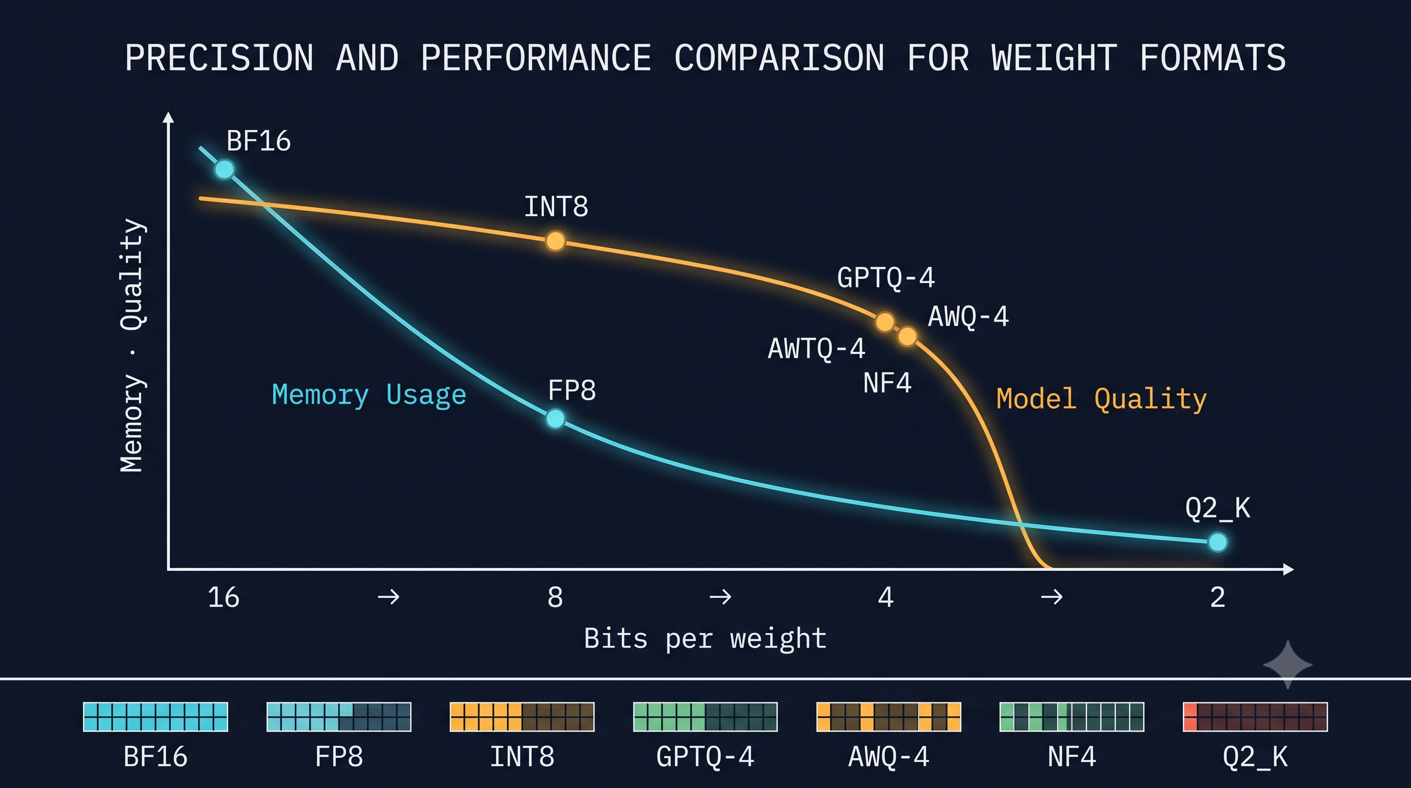
The Memory Wall Is the Inference Wall
The H100 SXM5 delivers 989 TFLOPS at FP16. Its HBM3 delivers 3.35 TB/s. The arithmetic ridge of the roofline — the intensity at which compute and bandwidth are co-equal constraints — sits at approximately 295 FLOPS/byte. Now consider autoregressive decode on a 70B-parameter model: at batch size 1, you load ~140 GB of weights per forward pass to generate a single token. The arithmetic intensity of this operation is vanishingly small — the model touches each weight once, executes a handful of multiply-accumulates, and discards it. You are running a 140 GB/step memory copy dressed up as inference.
This is the foundational fact: LLM decode is not compute-bound. It is memory-bandwidth-bound, almost definitionally. Every weight byte that can be eliminated from HBM traffic translates directly into more tokens per second — not through any clever scheduling, but because you are moving fewer bytes across the binding resource. If you cut weight precision from FP16 (2 bytes/weight) to INT4 (0.5 bytes/weight), you have, in principle, quadrupled your decode throughput ceiling. The tensor cores idle; the memory bus does not.
The second constraint is capacity, not bandwidth. A Llama 3.1 70B model in BF16 occupies ~140 GB — more than the 80 GB HBM of an H100. Serving it at FP16 requires two GPUs and NVLink tensor parallelism, with the attendant AllReduce overhead at every layer. At INT4 it fits on a single H100 with room for KV cache. Quantization does not merely speed up inference. At this model scale, it determines whether single-GPU serving is physically possible.
The combined argument: quantization is the primary lever for (a) fitting larger models into available HBM and (b) directly accelerating memory-bandwidth-bound decode by reducing bytes-per-weight. These are not competing benefits — they are the same physical phenomenon seen from different angles.
Part II — The Quantization Taxonomy
Dimensions of Variation
Every quantization scheme can be located on three axes: what is quantized, how many bits, and at what granularity.
What is quantized. Weight-only quantization stores weights at reduced precision and dequantizes them to FP16 on-the-fly before the matrix multiply. The activations remain in FP16. Weight-plus-activation quantization (WA) quantizes both, enabling fully integer matrix multiplications on hardware that supports them. The tradeoff is expressiveness versus hardware utilization: weight-only is more numerically forgiving (activations can be large and dynamic without loss), while W8A8 can exploit INT8 tensor-core throughput on Ampere and Hopper, yielding ~2× more compute TFLOPS if the kernel is fully implemented.
Bit width. The practical ladder runs W8 (INT8) → W4 (INT4) → W2 (INT2). Each halving roughly doubles the memory-bandwidth advantage and halves capacity requirements. Accuracy degradation is non-linear: W8 is nearly lossless on most models, W4 with calibration is within ~1–2 perplexity points on most language benchmarks, W2 requires aggressive algorithmic remediation (AQLM, QuIP#) and is not yet production-safe for general-purpose models.
Granularity. This is where most quality is won or lost at fixed bit width.
- Per-tensor: a single scale factor for the entire weight matrix. Cheapest to store, most aggressive approximation. Rarely used above W4.
- Per-channel (per-output-channel, or per-row): one scale factor per output channel. Captures inter-channel weight variation precisely. Standard for W8.
- Per-group (
group_size=128is the production consensus): the weight matrix is divided into contiguous groups of 128 elements, each with its own scale (and optionally zero-point). This subdivides the quantization problem into locally well-conditioned sub-problems, recovering most of the per-channel quality at a fraction of the parameter overhead. At W4 withgroup_size=128, the scale factors consume ~3% overhead on top of the 4-bit weights — negligible, and the quality delta versus per-channel is near-zero on all calibrated benchmarks.
The modern production answer for W4 is almost universally W4, per-group, group_size=128, because it is where quality, throughput, and storage cost intersect optimally.
Part III — Algorithms: How the Best Quantization Methods Work
GPTQ — Second-Order Weight Reconstruction
Paper: Frantar, E., Ashkboos, S., Hoefler, T., & Alistarh, D. (2022). GPTQ: Accurate Post-Training Quantization for Generative Pre-trained Transformers. arXiv:2210.17323.
GPTQ begins from a principled question: given that we must quantize each weight, which weights are most sensitive to error, and can we compensate for quantization error in one weight by adjusting others?
The answer comes from the Optimal Brain Surgeon framework. For each linear layer, GPTQ computes the layer-wise Hessian of the squared reconstruction error — specifically, the second-order term H = 2 X Xᵀ, where X is the layer’s input activations on a calibration corpus (typically 128 sequences from C4). The Hessian diagonal entry H_{ii} measures how sensitive the output error is to perturbation of weight w_i. GPTQ quantizes weights column by column in order of increasing sensitivity, and after quantizing each column, it applies a rank-1 update to the remaining unquantized weights to compensate for the induced error — a Cholesky-factored inverse-Hessian update that is numerically stable even for large matrices.
The practical output: W4 GPTQ quantized Llama 2 70B loses approximately 0.3–0.5 perplexity points on WikiText-2 versus the BF16 baseline. The calibration pass is offline and runs in 30–90 minutes on a single GPU depending on model size. At inference time, the model is statically INT4; dequantization to FP16 happens before each matrix multiply. This is weight-only quantization — activations remain FP16 — which means the TFLOPS savings from INT4 are not fully realized; what you recover is purely memory bandwidth and capacity.
GPTQ is the reference algorithm for post-training W4 quantization. Nearly all production W4 quantized models on Hugging Face (the GPTQ suffix models) are produced with it. vLLM and TensorRT-LLM both support GPTQ directly.
AWQ — Activation-Aware Weight Quantization
Paper: Lin, J., Tang, J., Tang, H., Yang, S., Dang, X., & Han, S. (2023). AWQ: Activation-aware Weight Quantization for LLM Compression and Acceleration. arXiv:2306.00978.
AWQ starts from an empirical observation that GPTQ implicitly discovers but does not exploit directly: a small fraction of weight channels — those corresponding to large activation magnitudes — disproportionately determine output quality. If 1% of weights are “salient” in this sense, quantizing them aggressively is catastrophic; protecting them is highly efficient.
AWQ’s mechanism: for each linear layer, measure the per-channel magnitude of input activations on a calibration set. Identify the top-1% salient input channels by activation scale. Rather than keeping these weights in FP16 (which would destroy the uniform bit-width and hardware efficiency), AWQ instead applies a per-channel scaling transformation before quantization: multiply salient weights by a scale factor s > 1 before quantizing to INT4, then divide by the same factor after dequantization. Because quantization error is proportional to the weight’s scale relative to the quantization step size, scaling up salient weights before quantization reduces their relative error — they occupy a larger fraction of the INT4 dynamic range. The non-salient weights absorb slightly more error, but their low activation magnitude means this has minimal impact on output.
This approach has three practical advantages over GPTQ: (1) no Hessian inversion is required, making calibration faster and more numerically stable; (2) the per-channel scales can be fused into preceding normalization layers at no runtime cost; and (3) it generalizes better across different calibration sets. AWQ benchmarks show marginally better perplexity than GPTQ on Llama 2 models at W4, particularly on instruction-tuned variants where the calibration-train split matters more. The llm-awq toolkit and AutoAWQ package are the standard implementations; both vLLM and TGI support AWQ inference natively.
GGUF and K-Quants — Ecosystem-Level Quantization
GGUF (GPT-Generated Unified Format) is the serialization format used by llama.cpp and its derivative ecosystem (Ollama, LM Studio, Jan). It is not an algorithm — it is a container format — but it bundles a family of quantization schemes called K-quants that are worth understanding in their own right.
K-quants (Q4_K, Q5_K, Q6_K, Q4_K_M, Q4_K_S) implement mixed-precision block quantization: within each 256-element block, the majority of weights are stored at the nominal bit width, but “super-blocks” encode scales and minimums at higher precision (typically FP16 or 6-bit). The _M (medium) and _S (small) suffixes indicate whether the attention and feed-forward layers use the same or slightly different precision within the model. Concretely:
- Q4_K_M: 4-bit weights with 6-bit scales per 32-element subblock; attention layers use Q6_K for the most sensitive weight matrices. Average effective bit width ~4.8 bits. Quality loss on Llama 2 70B: ~0.2 perplexity vs BF16 at 4.8 bits, comparable to GPTQ at the same effective width.
- Q5_K_M: Same structure at 5-bit nominal; ~5.7 effective bits; within ~0.05 perplexity of BF16 on most benchmarks.
- Q6_K: 6-bit weights; effectively lossless on nearly all models; ~6.6 effective bits with scales.
K-quants are CPU-optimized first — they include hand-vectorized AVX2 and ARM NEON kernels — but llama.cpp now includes CUDA backends. For consumer GPU inference (RTX 4090, 3090, consumer-tier deployment), GGUF Q4_K_M has emerged as the de facto standard: it produces near-GPTQ quality, loads into 24 GB VRAM, and runs without any proprietary toolkit dependency.
The critical distinction: GGUF/K-quants are optimized for the llama.cpp stack. If you are deploying on H100 with vLLM or TRT-LLM, GPTQ or AWQ will outperform them because the GPU-native kernels (marlin, exllamav2, cutlass W4A16) are far more optimized for server-grade hardware than GGUF’s CUDA path.
FP8 — Native Hopper Hardware Quantization
FP8 is not post-hoc compression. It is a first-class hardware precision format introduced in the H100’s fourth-generation Tensor Engine — the first NVIDIA GPU with native FP8 matrix arithmetic.
FP8 exists in two variants with different numerical properties: E4M3 (4 exponent bits, 3 mantissa) and E5M2 (5 exponent bits, 2 mantissa). E4M3 provides finer precision and a narrower dynamic range; it is used for forward-pass weights and activations where precision matters. E5M2 has a wider dynamic range but coarser precision; it is preferred for backward-pass gradients, which can span many orders of magnitude.
At inference, the standard configuration is W8A8 FP8: both weights and activations stored as E4M3, with FP8 tensor-core matrix multiplies accumulating in FP32. The H100 delivers approximately 3,979 TFLOPS at FP8 sparse — roughly 2× the FP16 throughput — because the same number of tensor-core cycles processes twice as many operands per word. This is the only path to beating FP16 on compute throughput (rather than bandwidth), because the TFLOPS actually double when the hardware arithmetic is FP8 vs FP16.
The NVIDIA Transformer Engine handles FP8 transparently at the framework level: it maintains FP16 master weights, selects per-tensor scaling factors via a history-based algorithm, and casts to FP8 at the matrix multiply boundary. For inference, the Transformer Engine in TensorRT-LLM automates this entirely. The principal accuracy risk: FP8 E4M3 has a maximum representable value of 448; models with large activation outliers (particularly after layer normalization) can overflow without careful per-tensor or per-channel scaling calibration. The Transformer Engine handles this through delayed scaling with amax history buffers.
On the B200 (Blackwell), FP4 (E2M1) is additionally available, doubling FP8 throughput again at the cost of more aggressive quantization. FP4 requires TensorRT Model Optimizer and is not yet supported in mainline vLLM; accuracy validation on specific model families is mandatory before production deployment.
NF4 — Normal Float for QLoRA Fine-Tuning
Paper: Dettmers, T., Pagnoni, A., Holtzman, A., & Zettlemoyer, L. (2023). QLoRA: Efficient Finetuning of Quantized LLMs. arXiv:2305.14314.
NF4 (NFloat4) is a 4-bit data type designed by Dettmers et al. with a specific insight: the weights of a pretrained neural network, after normalization, follow an approximately normal distribution. Standard integer quantization distributes quantization levels uniformly — equal spacing between 0 and the maximum value — which wastes precision in the sparse tails of the weight distribution and over-allocates it near the extremes.
NF4 instead distributes quantization levels to be information-theoretically optimal for the normal distribution: the 16 representable values (in 4 bits) are placed at the 1/17, 2/17, …, 16/17 quantiles of N(0,1). This is not a uniform grid. Values cluster densely near zero — where most weights live — and spread sparsely at the tails. For a normally distributed weight tensor, this minimizes expected quantization error relative to any other 4-bit scheme.
The implementation in bitsandbytes (the standard QLoRA library) combines NF4 weights with double quantization: the quantization constants themselves are quantized to FP8, saving an additional 0.37 bits per parameter on average. In practice, a 65B-parameter model in NF4 + double quantization occupies approximately 33 GB — fitting on a single 40 GB A100 for fine-tuning with LoRA adapters.
A critical distinction from GPTQ and AWQ: NF4 is a training-time quantization scheme designed for QLoRA fine-tuning, not a production inference format. The bitsandbytes kernel does not match the throughput of marlin or exllamav2 W4A16 kernels. For the fine-tuning workflow, NF4 is the correct choice. For deployment after fine-tuning, the merged adapter should be re-quantized with GPTQ or AWQ using a task-specific calibration set.
Part IV — The Decision Matrix
The following matrix encodes hard-won production experience across the primary deployment configurations. Use it as a first-order filter; validate accuracy on your specific model and task distribution before committing.
By Inference Engine
| Method | vLLM | TensorRT-LLM | llama.cpp | Notes |
|---|---|---|---|---|
| GPTQ (W4A16) | ✅ Native (marlin kernel) | ✅ Native | ⚠️ Partial | Marlin kernel requires Ampere+; significant speedup over naive dequant |
| AWQ (W4A16) | ✅ Native | ✅ Native | ⚠️ Via conversion | AutoAWQ → GPTQ bridge exists; quality preserved |
| GGUF Q4_K_M | ❌ Not supported | ❌ Not supported | ✅ Primary format | Do not force GGUF into server-grade GPU serving stacks |
| FP8 (E4M3) | ✅ (H100/B200 only) | ✅ (Transformer Engine) | ❌ No FP8 | Requires Hopper or Blackwell; hardware-accelerated |
| NF4 | ⚠️ Via bitsandbytes | ❌ | ❌ | Training use only; throughput below GPTQ at same bit width |
| BF16 (baseline) | ✅ | ✅ | ✅ | Reference point; use when VRAM is unconstrained |
By Hardware Target
| Hardware | Recommended Method | Rationale |
|---|---|---|
| H100 / A100 (server, 70B+) | FP8 W8A8 (TRT-LLM) or W4A16 GPTQ/AWQ (vLLM) | FP8 is the throughput ceiling; W4 if VRAM is primary constraint |
| H200 (server, 70B+) | FP8 or BF16 | 141 GB HBM accommodates Llama 3.1 70B at BF16 with KV cache headroom; FP8 for throughput |
| B200 / GB200 (server, 405B+) | FP4 (TRT-LLM + TensorRT Model Optimizer) | Doubles FP8 throughput; validate accuracy first |
| RTX 4090 / 3090 (consumer 24 GB) | GGUF Q4_K_M (llama.cpp / Ollama) | Highest quality/throughput on consumer stack; llama.cpp CUDA kernels well-optimized |
| RTX 4090 (vLLM deployment) | AWQ W4A16 or GPTQ W4A16 | If running vLLM on consumer hardware; avoid GGUF |
| Apple Silicon (M2/M3 Ultra) | GGUF Q4_K_M or Q5_K_M | llama.cpp Metal backend; K-quants well-supported |
| Multi-GPU A100 cluster (fine-tuning) | NF4 + QLoRA | Memory efficiency during training; re-quantize with GPTQ post-merge |
By Workload
| Workload | Priority | Recommended Path |
|---|---|---|
| Production inference, throughput-maximized (H100) | Tokens/sec, cost/token | FP8 via TRT-LLM; if engine constraints, GPTQ/AWQ via vLLM |
| Production inference, latency-critical (TTFT) | Time-to-first-token | FP8 W8A8 — full tensor-core utilization; prefill is compute-bound |
| Single-GPU serving (fits in 80 GB) | Model size ≤ ~40B at BF16 | BF16 or FP8; no W4 needed |
| Single-GPU serving (70B on H100) | Must fit in 80 GB | W4A16 GPTQ or AWQ, group_size=128 |
| Consumer deployment (any 70B model) | Accessibility | GGUF Q4_K_M (fits in 40–48 GB VRAM or fast CPU+GPU split) |
| QLoRA fine-tuning (any scale) | Training memory | NF4 (bitsandbytes), re-quantize for deployment |
| Research / ablation | Reproducibility | GPTQ (most documented, most cited, widest baseline coverage) |
Accuracy Retention (WikiText-2 Perplexity, Llama 2 70B, approximate)
| Method | Effective Bits | PPL Δ vs BF16 |
|---|---|---|
| BF16 | 16 | 0 (baseline) |
| FP8 E4M3 | 8 | ~0.01–0.05 |
| W8 per-channel | 8 | ~0.05 |
| GPTQ W4 gs=128 | ~4.1 | ~0.3–0.5 |
| AWQ W4 gs=128 | ~4.1 | ~0.25–0.45 |
| GGUF Q4_K_M | ~4.8 | ~0.2–0.3 |
| GGUF Q5_K_M | ~5.7 | ~0.05–0.1 |
| NF4 (bitsandbytes) | ~4.5 | ~0.3–0.5 |
| W2 (uncompensated) | 2 | >5 (task-dependent failure) |
Part V — Production Engineering Notes
Calibration Set Selection Is Not Trivial
GPTQ and AWQ both require a calibration corpus: a sample of text that estimates the activation statistics the model will see at runtime. The standard choice — 128 sequences from C4 — is appropriate for general-purpose models. For instruction-following models, code generation specialists, or models that will primarily see a domain-specific distribution (legal text, medical literature, structured data), re-calibrating on domain-representative data consistently recovers 0.1–0.3 perplexity points versus the C4 default. This is especially important for AWQ, which uses activation magnitudes directly to identify salient channels; a mismatched calibration set will misidentify salience.
KV Cache Quantization Is a Separate Problem
Weight quantization addresses the parameter bytes. The KV cache — which at batch=32, context=8K for Llama 3 70B occupies ~40 GB on a single H100 — is a distinct memory consumer. Modern serving stacks (vLLM ≥ 0.4, TRT-LLM 0.9+) support INT8 or FP8 KV cache quantization independently of weight precision. For long-context serving, this can be as impactful as W4 weights. The two should be configured together as a system, not as independent decisions.
The Outlier Problem
Large language models exhibit activation outliers — a phenomenon first characterized at scale in LLM.int8() (Dettmers et al., 2022) — where a small number of embedding dimensions exhibit values 100× larger than the median. These outliers appear systematically in models trained beyond ~6.7B parameters and make symmetric per-tensor quantization of activations catastrophically lossy. This is the reason W4A8 and W4A4 schemes are so much harder than W4A16: weights are approximately normally distributed and calibrate well; activations are not. Methods that successfully handle activation quantization (SmoothQuant, QuIP#, AQLM) do so by migrating outlier scaling difficulty from activations into weights via mathematically equivalent transformations. For any WA scheme, assume outlier handling is necessary and verify it is implemented in your chosen toolkit before deployment.
References
- Frantar, E., Ashkboos, S., Hoefler, T., & Alistarh, D. (2022). GPTQ: Accurate Post-Training Quantization for Generative Pre-trained Transformers. arXiv:2210.17323.
- Lin, J., Tang, J., Tang, H., Yang, S., Dang, X., & Han, S. (2023). AWQ: Activation-aware Weight Quantization for LLM Compression and Acceleration. arXiv:2306.00978.
- Dettmers, T., Pagnoni, A., Holtzman, A., & Zettlemoyer, L. (2023). QLoRA: Efficient Finetuning of Quantized LLMs. arXiv:2305.14314.
- Dettmers, T., Lewis, M., Belkada, Y., & Zettlemoyer, L. (2022). LLM.int8(): 8-bit Matrix Multiplication for Transformers at Scale. arXiv:2208.07339.
- NVIDIA. (2022). NVIDIA H100 Tensor Core GPU Architecture Whitepaper.
- NVIDIA. (2024). NVIDIA Blackwell Architecture Technical Brief.
- Hassibi, B., & Stork, D. G. (1992). Second Order Derivatives for Network Pruning: Optimal Brain Surgeon. NeurIPS 1992. (Theoretical basis for GPTQ’s Hessian-aware framework.)
- Kwon, W., Li, Z., Zhuang, Y., et al. (2023). Efficient Memory Management for Large Language Model Serving with PagedAttention. SOSP 2023. (Context for KV cache quantization importance.)
BibTeX
@article{fp4-2606019,
  title   = {The Inference Engineer's Definitive Guide to Quantization},
  author  = {fp4 editorial desk},
  year    = {2026},
  url     = {https://fp4.dev/algorithm/quantization-inference-guide/},
  journal = {fp4}
}