Preface: The Fundamental Asymmetry That Makes Everything Possible
There is a profound and exploitable asymmetry at the heart of transformer inference that most engineers glance past without recognizing its engineering worth. It takes roughly the same amount of wall-clock time for a large language model to verify a sequence of tokens as it does to generate a single one. This is not a quirk — it is a structural consequence of how matrix multiplications parallelize across the sequence dimension. Speculative decoding is the discipline of weaponizing this asymmetry into measurable, provable speedup without altering a single probability the target model assigns.
This article is a rigorous dissection — not a survey. We will derive, not merely describe.
1. The Core Insight: Draft Fast, Verify in Parallel
The foundational papers — Leviathan et al. (2023) “Fast Inference from Transformers via Speculative Decoding” (arXiv:2211.17192) and Chen et al. (2023) “Accelerating Large Language Model Decoding with Speculative Sampling” — arrived simultaneously and independently, which is always a sign that an idea is structurally inevitable.
The setup is deceptively simple. You have a large target model — the one whose distribution you care about — and a small, cheap draft model . The draft model is fast because it is small: fewer parameters, fewer layers, lower hidden dimension. The target model is slow because it is large: this is the model actually serving your quality requirements.
The algorithm proceeds in three stages per decoding step:
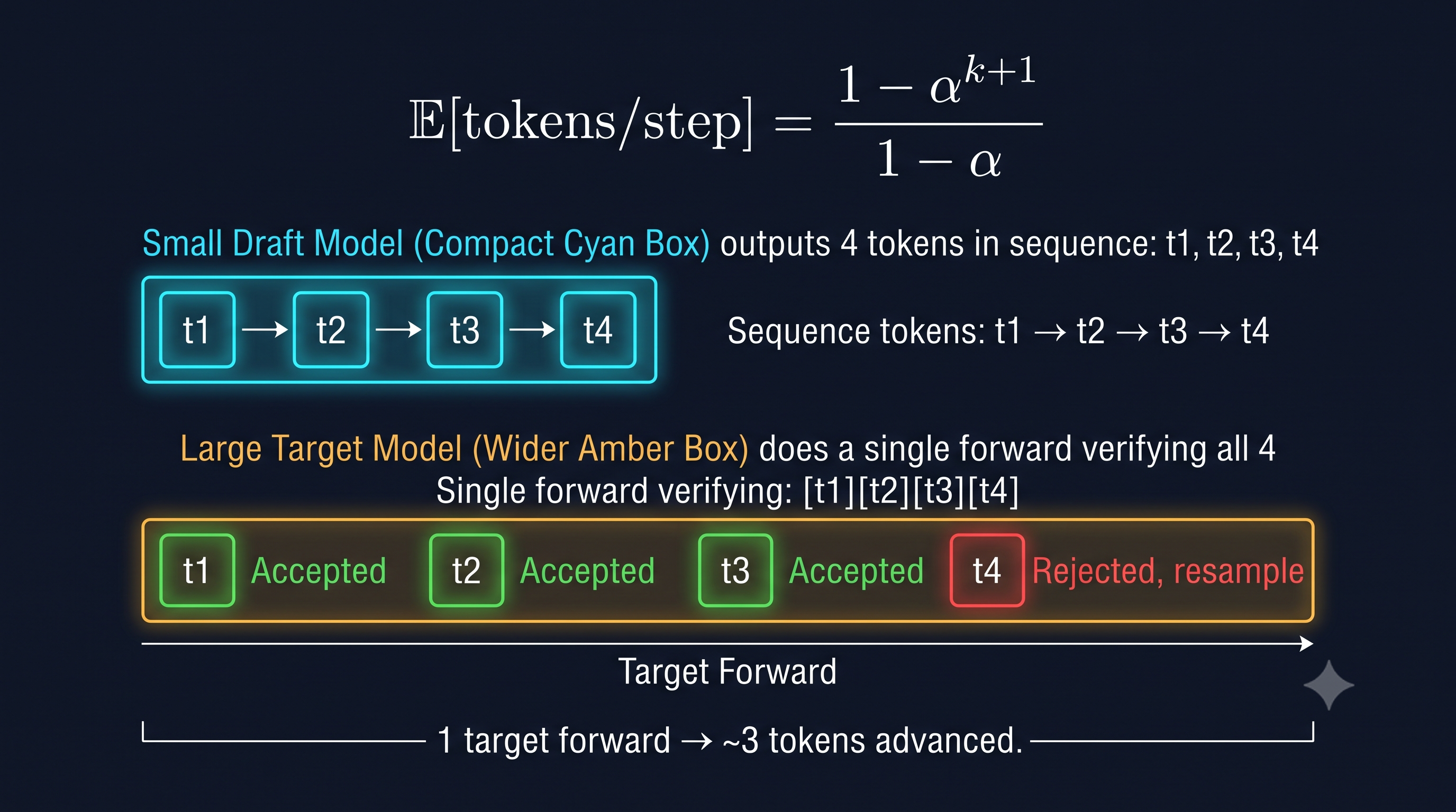
Stage 1 — Draft Generation: The small model autoregressively generates candidate tokens , producing draft probabilities at each position. This runs serially, but because is tiny, it is cheap. Think of this as a speculative bet placed in milliseconds.
Stage 2 — Parallel Verification: A single forward pass of the target model is executed over the extended context . Because the transformer attention is computed over all positions simultaneously, this single pass yields target probabilities for all draft positions in parallel. The arithmetic here is critical: one forward pass of over tokens costs approximately the same as one forward pass over tokens in terms of KV-cache amortized cost, because the batch dimension and the sequence-parallel structure of matrix multiplication absorb the extra positions at near-zero marginal cost.
Stage 3 — Token Selection: Each draft token is accepted or rejected using a modified rejection sampling rule (derived in Section 2). The longest accepted prefix is kept, and the next token after the first rejection is resampled from a corrected distribution. In the best case, all tokens are accepted and one bonus token is generated for free; in the worst case, the first draft token is rejected and we have recovered a single target-distribution token at a cost roughly equivalent to two forward passes.
The insight crystallizes to this: the target model’s verification cost per token decreases as more draft tokens are accepted, because the fixed overhead of a forward pass is amortized over the entire accepted prefix.
2. Why It Is Lossless: The Modified Rejection Sampling Rule
This section is where most explanations fail the reader. Speculative decoding is not approximate. It produces samples that are identically distributed to samples drawn directly from . The proof is constructive, through a modified rejection sampling scheme.
Let denote the target probability for token at a given position, and the draft probability. A draft token is accepted with probability:
If rejected, a new token is drawn from the residual distribution:
where normalizes to a valid probability distribution.
Proof of losslessness: The probability of outputting token through this scheme is:
The first term captures acceptance: the draft proposes with probability and it is accepted with probability . The second term captures rejection followed by resampling from .
Simplifying the first term: .
The rejection probability for any single draw is . And where .
Note that by conservation of probability mass. Therefore:
The algebra is clean, the result is exact. No approximation is made. The output distribution is — the target model’s distribution — whether we accepted the draft token or resampled. This is why speculative decoding can be deployed in production without any quality regression; it is a pure inference acceleration technique.
3. The Speedup Formula: When the Math Pays Off
Let denote the token-level acceptance rate — the probability that a given draft token is accepted. For a draft length of , the expected number of tokens generated per decoding step is:
This is derived from the geometric series for the expected accepted prefix length. If all tokens are accepted with probability independently:
- With probability , all tokens are accepted and a bonus token is sampled: tokens total.
- With probability , the -th token is the first rejection: tokens total.
Summing:
Now, the speedup ratio relative to vanilla autoregressive decoding (1 token per forward pass of ) is:
where accounts for the overhead of running drafting plus any memory bandwidth cost. In practice, – for well-chosen draft models (7B target, 160M draft), making the denominator –.
Regime analysis:
| Tokens/Step | Tokens/Step | Practical Speedup | |
|---|---|---|---|
| 0.5 | 1.94 | 1.99 | ~1.5–1.7× |
| 0.7 | 2.76 | 3.28 | ~2.1–2.6× |
| 0.85 | 3.50 | 4.76 | ~2.8–3.8× |
| 0.95 | 4.40 | 7.10 | ~3.5–5.5× |
The formula reveals a critical threshold: speculative decoding pays off only when . For draft tokens and overhead factor , break-even occurs near . In practice, a well-matched draft model operating on natural language achieves , placing typical deployments comfortably in the profitable regime.
Note also the saturation effect: increasing beyond a certain point yields diminishing returns because and the formula plateaus at . The optimal balances the length of the speculative window against the probability of early rejection wasting draft compute.
4. When Speculative Decoding Does Not Help
Understanding the failure modes is as important as understanding the wins. There are three structural regimes where speculative decoding delivers no benefit, and deploying it blindly in these regimes wastes engineering capital.
Failure Mode 1: Low Acceptance Rate ()
If the draft model’s predictions are systematically misaligned with the target’s distribution — because the task demands complex reasoning, the domain is highly specialized, or the draft model is too small to track the target’s token preference — then collapses. At with , the expected tokens per step is only , while we’ve incurred the full overhead of draft generation and parallel verification. The system is slower than vanilla decoding. This manifests acutely on tasks like formal mathematics, code generation in obscure languages, or multilingual reasoning where small draft models diverge rapidly.
Failure Mode 2: GPU Already Saturated (Batch Inference)
The speedup argument depends on the parallel verification pass costing approximately the same as a single-token generation pass. This holds only when the GPU’s arithmetic units are not already saturated by the batch dimension. At large batch sizes (B ≥ 32 on modern A100s), forward passes are compute-bound — the matrix multiplications are running at near-peak FLOP utilization. Adding extra sequence positions does not “come for free”; it linearly increases the compute cost. In this regime, speculative decoding offers zero speedup and may introduce latency regression due to speculative token management overhead. This is a fundamental point: speculative decoding is a memory-bandwidth optimization, not a compute optimization. It exploits the bandwidth-bound, small-batch regime where the GPU has spare arithmetic capacity.
Failure Mode 3: Latency-Insensitive Batch Workloads
Batch processing pipelines optimizing for throughput (tokens per second per dollar) rather than time-to-first-token or end-to-end latency do not benefit from speculative decoding’s structure. High-throughput offline inference is already using maximum batch sizes to saturate GPU utilization — exactly the regime described above. Moreover, the draft model adds memory pressure (additional KV cache, additional weight loading), reducing the maximum achievable batch size and potentially decreasing throughput.
5. Variants: The Architecture of Speculation
The success of the original formulation has catalyzed a family of architectures, each attacking the core bottleneck from a different angle.
Medusa — Multi-Head Drafting Within the Same Model
Reference: arXiv:2401.10774 (Cai et al., 2024)
Medusa eliminates the separate draft model entirely. Instead, multiple lightweight “Medusa heads” are attached to the final hidden layer of the target model. Each head is a small feed-forward network that predicts one token ahead in the future sequence: head predicts the token at position independently of other heads. During inference, a single forward pass of the target model simultaneously produces standard output logits and draft predictions from all Medusa heads.
This is architecturally elegant because: (a) the draft inference cost collapses to near-zero — it is a byproduct of the target’s forward pass; (b) there is no KV-cache management split between two models; (c) the acceptance rates are typically high because the heads condition on the exact same hidden representations as the target’s own sampling.
The trade-off: Medusa requires fine-tuning the target model to train the auxiliary heads, and the heads use independent prediction (ignoring inter-head dependencies), limiting acceptance rates on longer speculative windows. The paper reports 2.2–3.6× speedup on Vicuna models with negligible quality loss.
Eagle — Feature-Level Autoregression
Reference: arXiv:2401.15077 (Li et al., 2024)
Eagle addresses Medusa’s independence assumption. Rather than predicting future tokens from fixed position-independent heads, Eagle trains a lightweight draft model that performs autoregression at the feature level — that is, in the hidden state space of the target model rather than the token space.
Concretely, Eagle’s draft model takes the target model’s penultimate hidden states as input (not just the token embeddings) and autoregressively predicts the next hidden state, from which token probabilities are derived. This is profound: hidden states encode far richer contextual information than token IDs. The draft operates with significantly more signal per step, leading to substantially higher acceptance rates — the paper demonstrates on many tasks, pushing speedups to 3–4× on commodity hardware.
Eagle requires the target model to expose its intermediate activations, making it slightly more invasive than external draft approaches, but less invasive than Medusa’s head fine-tuning.
Lookahead Decoding — Jacobi Iteration and N-Gram Caches
Lookahead decoding takes an entirely different philosophical approach, borrowing from numerical methods. Rather than using a small draft model, it applies a Jacobi iteration strategy: multiple token positions are decoded in parallel at each step using the current context, producing a fixed-point solution through iterative refinement. Token candidates from this parallel decoding are cached as n-grams, and future steps retrieve matching n-gram continuations as draft sequences, bypassing any neural draft model entirely.
The advantage: zero additional model parameters, zero additional training. The disadvantage: acceptance rates are task-dependent and often lower than learned draft models, and the n-gram cache introduces memory overhead that must be managed carefully in production.
6. Production Engineering: Where Speculation Wins and How to Deploy It
The theoretical analysis points unambiguously to the optimal deployment context: low-batch, latency-sensitive, online serving.
Concretely, this means:
- Batch size , ideally (single-user, interactive generation)
- Sequences where the draft model’s training domain overlaps significantly with query distribution (general-purpose chatbots, coding assistants in mainstream languages)
- Target models in the 13B–70B parameter range, paired with 1B–7B draft models from the same model family (same tokenizer, similar pretraining distribution is critical)
For production deployment, three engineering decisions dominate performance:
Draft model selection: The draft must be from the same family as the target (e.g., LLaMA-3-70B with LLaMA-3-8B as draft) to ensure tokenizer identity and distributional alignment. A cross-family pair will suffer catastrophic acceptance rate degradation. The ratio of target-to-draft parameters should be in the range 8:1 to 70:1; lower than 8:1 and the draft cost is non-negligible; higher than 70:1 and the acceptance rate collapses.
Draft length calibration (): The optimal should be calibrated empirically per task domain. Interactive chat might optimally use ; code generation where sequences are more predictable might use ; mathematical reasoning where the target diverges sharply from draft might use . Adaptive — reducing draft length when recent acceptance rates are low — is a valuable production optimization.
KV-cache management: In speculative decoding, the target model’s KV cache must be truncated upon rejection — the cached keys and values for rejected positions must be evicted. This introduces write operations into an otherwise append-only cache. High-performance implementations (e.g., vLLM’s speculative decoding backend) handle this with copy-on-write semantics or slot reservation, but naive implementations see significant overhead from cache rollback.
At scale, speculative decoding is often combined with tensor parallelism for the target model and no parallelism for the draft model (which is small enough to run on a single GPU). The pipeline runs draft generation on one GPU while the target model occupies a tensor-parallel group — hiding the draft latency almost entirely within the target’s memory transfer cycles.
7. The Deeper Principle: Computation as a Temporal Resource
Speculative decoding is, at its philosophical core, about temporal arbitrage. The target model’s forward pass represents fixed wallclock time — paid whether 1 token or tokens are verified. The draft model runs fast enough that its cost is a fraction of that fixed overhead. The modified rejection sampler is the arbitration mechanism that ensures this temporal arbitrage produces no distributional distortion.
The result is a system that provably delivers the target model’s quality at empirically 2–4× the throughput on latency-sensitive workloads. In an era where inference costs dominate LLM economics at scale, this is not a research curiosity — it is engineering leverage of the highest order.
The lineage from Leviathan et al. through Medusa and Eagle represents not incremental refinement but a deepening understanding of the asymmetries in transformer computation: the asymmetry between sequence position and batch dimension, the asymmetry between generation cost and verification cost, the asymmetry between token space and hidden state space as domains for speculation. Each new variant exploits a different facet of the same underlying geometry.
The trajectory is clear: as models grow larger and serve more latency-sensitive applications, speculative decoding — in its increasingly sophisticated forms — will become as standard as KV caching in production inference stacks.
References
-
Leviathan, Y., Kalman, M., & Matias, Y. (2023). Fast Inference from Transformers via Speculative Decoding. arXiv:2211.17192.
-
Chen, C., Borgeaud, S., Irving, G., Lespiau, J., Sifre, L., & Jumper, J. (2023). Accelerating Large Language Model Decoding with Speculative Sampling. DeepMind Technical Report.
-
Cai, T., Li, Y., Geng, Z., Peng, H., & Dao, T. (2024). Medusa: Simple LLM Inference Acceleration Framework with Multiple Decoding Heads. arXiv:2401.10774.
-
Li, Y., Wei, F., Zhang, C., & Zhang, H. (2024). Eagle: Speculative Sampling Requires Rethinking Feature Uncertainty. arXiv:2401.15077.
BibTeX
@article{fp4-2606016,
  title   = {Speculative Decoding: The Physics of Stolen Time in Autoregressive Inference},
  author  = {fp4 editorial desk},
  year    = {2026},
  url     = {https://fp4.dev/algorithm/speculative-decoding/},
  journal = {fp4}
}