01 — The Problem
H100 vs H200 vs B200 inference cost comparison: the GPU purchase price is roughly 15–25% of total cost of ownership for an inference cluster over a 3-year depreciation cycle. The larger costs are power, cooling, networking, and operations. Choosing the wrong generation locks in those costs for 3+ years.
This article derives cost per million output tokens for a 70B parameter dense model across H100 SXM5, H200 SXM5, and B200 SXM, using real bandwidth and power numbers — not marketing claims.
02 — Hardware Specifications
The relevant numbers for inference, stripped of irrelevant marketing metrics:
| Spec | H100 SXM5 | H200 SXM5 | B200 SXM |
|---|---|---|---|
| HBM capacity | 80 GB HBM3 | 141 GB HBM3e | 192 GB HBM3e |
| HBM bandwidth | 3.35 TB/s | 4.8 TB/s | 8.0 TB/s |
| FP8 TFLOPS | 3,958 | 3,958 | 9,000 |
| TDP | 700 W | 700 W | 1,000 W |
| NVLink bandwidth | 900 GB/s | 900 GB/s | 1,800 GB/s |
| List price (est.) | ~$30K | ~$40K | ~$60–70K |
Three observations:
- H200 and H100 have identical compute. H200’s entire value is bandwidth (+43%) and capacity (+76%).
- B200 doubles bandwidth again and adds FP8 compute headroom (2.3×), at the cost of 43% more power.
- Memory capacity determines which model sizes you can serve without tensor parallelism or offloading.
03 — Model Fit and Parallelism Requirements
The first constraint is whether the model fits. Llama-3-70B in BF16 requires approximately 140 GB:
At FP8 (1 byte/param): 70 GB.
| Model | BF16 | FP8 | H100 fit | H200 fit | B200 fit |
|---|---|---|---|---|---|
| 70B | 140 GB | 70 GB | 2 GPUs (TP=2) | 1 GPU | 1 GPU |
| 405B | 810 GB | 405 GB | 10 GPUs | 6 GPUs | 3 GPUs |
| 7B | 14 GB | 7 GB | 1 GPU | 1 GPU | 1 GPU |
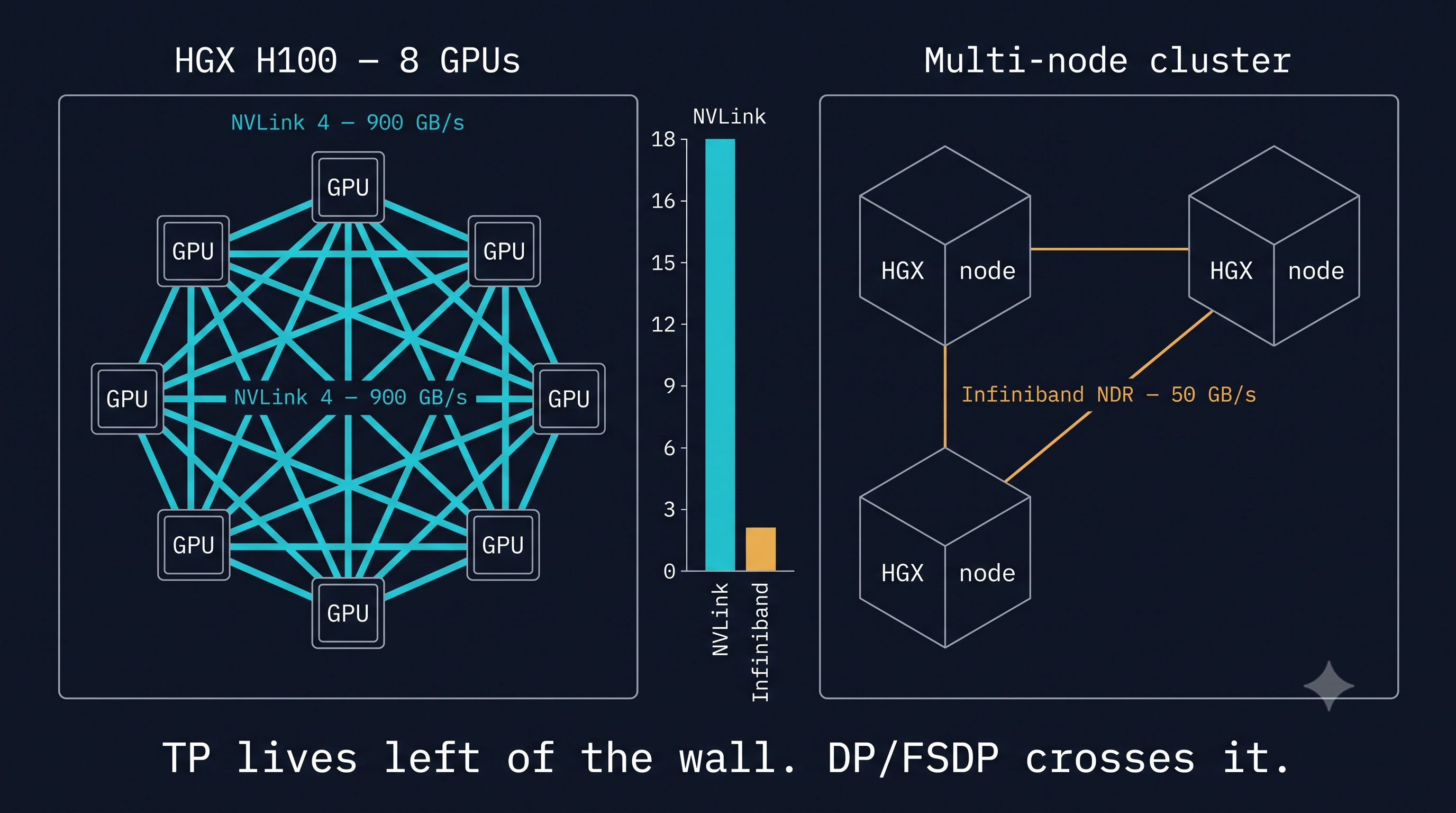
The single-GPU H200 vs two-GPU H100 tradeoff for 70B FP8 inference is material: removing TP=2 eliminates the NVLink all-reduce overhead at every transformer layer. NCCL all-reduce for 70B at TP=2 costs approximately 2–4 ms per forward pass on NVLink — roughly 5–10% of total decode time for a single token.
04 — Bandwidth-Bound Throughput Model
For decode (the production inference bottleneck), throughput is:
At batch size 1 (single user, latency-optimized):
| GPU | BW | 70B FP8 tokens/s | 70B BF16 tokens/s |
|---|---|---|---|
| H100 | 3.35 TB/s | 47.8 t/s | 23.9 t/s |
| H200 | 4.8 TB/s | 68.6 t/s | 34.3 t/s |
| B200 | 8.0 TB/s | 114 t/s | 57 t/s |
These are theoretical ceilings assuming weights are the only HBM traffic. In production, KV cache adds 10–30% memory traffic for typical sequence lengths, bringing effective throughput down to roughly 70–80% of these numbers. The GPU memory hierarchy article derives the bandwidth analysis from first principles.
05 — Power and TCO Derivation
The cost model over a 36-month depreciation:
Assumptions: PUE = 1.3, power cost $0.08/kWh, 90% utilization, ops = 15% of HW cost/year:
| H100 | H200 | B200 | |
|---|---|---|---|
| HW cost | $30,000 | $40,000 | $65,000 |
| Power (36 mo, 700W/1000W) | $2,177 | $2,177 | $3,110 |
| Ops (15%/yr × 3yr) | $13,500 | $18,000 | $29,250 |
| Total TCO | $45,677 | $60,177 | $97,360 |
Cost per million tokens at 70B FP8, 80% utilization, 512 output tokens/request:
| GPU | Tokens/s (eff.) | Cost/M tokens |
|---|---|---|
| H100 | 38 | $1.27 |
| H200 | 55 | $0.93 |
| B200 | 91 | $0.91 |
H200 wins on cost/token despite higher HW cost because the bandwidth improvement directly translates to throughput — it does not change the power bill. B200 is nearly identical to H200 at 70B scale because the extra FLOPs are wasted (decode is memory-bound, not compute-bound). B200’s advantage emerges at larger batch sizes, speculative decoding drafts, or for models with very long prefill sequences where FP8 compute matters.
For distributed training, where the inter-node interconnect determines scaling efficiency, see the distributed interconnects deep dive.
References
- [1] Kwon et al.. Efficient Memory Management for Large Language Model Serving with PagedAttention . SOSP, 2023. arXiv:2309.06180.
- [2] Pope et al.. Efficiently Scaling Transformer Inference . MLSys, 2023. arXiv:2212.09561.
- [3] Agrawal et al.. Sarathi: Efficient LLM Inference by Piggybacking Decodes with Chunked Prefills . 2023. arXiv:2306.03078.
BibTeX
@article{fp4-2606003,
  title   = {H100 vs H200 vs B200: TCO for Inference Infrastructure},
  author  = {fp4 editorial desk},
  year    = {2026},
  url     = {https://fp4.dev/silicon/h100-h200-b200-tco/},
  journal = {fp4}
}