Preface: Why This Guide Exists
Every distributed training paper describes its parallelism strategy in the methodology section. None of them tells you how they chose it — the reasoning that connects hardware topology, model architecture, memory budget, and batch size into a concrete configuration. The Megatron-LM papers give you the formulas. The DeepSeek-V3 report gives you the outcome. What’s missing is the decision tree that gets you from “I have a 70B model and a 64-GPU pod” to “here is what I run, and here is why everything else would have been slower or infeasible.”
This guide fills that gap.
The foundational constraint, which no degree of engineering ingenuity escapes, is the bandwidth hierarchy. NVLink 4 on an H100 node delivers 900 GB/s bidirectional between GPUs on the same chassis. InfiniBand NDR, connecting nodes across the fabric, delivers 50–100 GB/s aggregate per node. The ratio is roughly 9–18×. Every parallelism decision is, at its core, a negotiation with that ratio: keep the expensive collectives inside the fast domain, push the cheap ones (or the overlappable ones) across the slow domain.
1. Tensor Parallelism (Megatron-Style)
The Mechanics
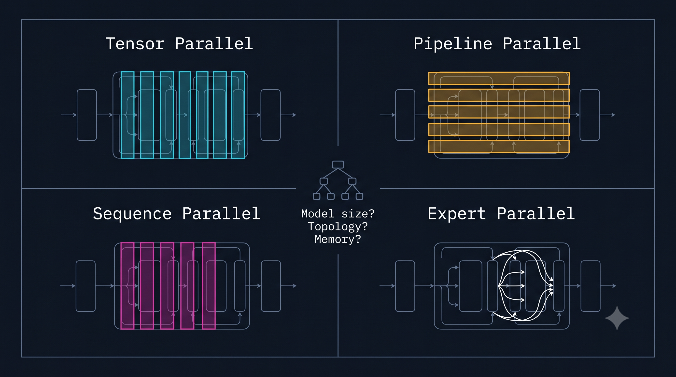
Tensor parallelism (TP), formalized by Shoeybi et al. in Megatron-LM (arXiv:1909.08053), partitions individual weight matrices across tp_degree GPUs. The standard scheme applied to a transformer MLP with weight matrices A ∈ ℝ^{h × 4h} and B ∈ ℝ^{4h × h}:
Column-parallel (A): Partition A column-wise. Each GPU i holds A_i ∈ ℝ^{h × (4h/tp)}. Given input X ∈ ℝ^{batch × h}, each GPU independently computes its local output Y_i = X · A_i, producing partial activations of width 4h/tp. No communication required at this step — each GPU received the full X from the previous AllReduce.
Row-parallel (B): Partition B row-wise. Each GPU i holds B_i ∈ ℝ^{(4h/tp) × h}. Each GPU computes its partial output Z_i = Y_i · B_i ∈ ℝ^{batch × h}. This is a partial sum — correct output requires summing across all tp_degree shards.
AllReduce: A single AllReduce over the tp_degree GPUs reduces the partial sums into the complete output Z = Σ Z_i.
The attention block mirrors this pattern: Q, K, V projections are column-parallel (split by head), the output projection is row-parallel. Two AllReduces per transformer block, eight AllReduces per four-layer pipeline stage.
The Communication Budget
For a forward pass with hidden dimension h = 8192, batch size B = 4096 tokens, and tp = 8:
AllReduce tensor size = B × h × 2 bytes (bfloat16) = 4096 × 8192 × 2 = 64 MBAllReduce time (NVLink 4, ring, 7/8 efficiency) ≈ 2 × (7/8) × 64 MB / 450 GB/s ≈ 0.25 msAgainst a compute time of ~2–4 ms per block on 8 H100s: overhead is 6–12%. Acceptable. On InfiniBand NDR at 50 GB/s per NIC, the same AllReduce takes 1.75–2.5 ms — exceeding the compute time itself. This is the hard constraint that pins TP inside a single NVLink domain. Megatron-LM (§4 of 1909.08053) makes this restriction explicit; it remains correct on every subsequent hardware generation.
What TP Buys You
TP shards both compute and memory. Each GPU holds 1/tp of every weight matrix, so peak weight memory scales as O(P/tp). Critically, the intermediate activations within the MLP (the 4h width intermediate) exist at 1/tp scale per GPU. At tp = 8 on a 70B model with h = 8192, the intermediate activation of 4h = 32768 per token is 32,768/8 = 4,096 per GPU — a meaningful reduction that allows larger batch sizes.
2. Pipeline Parallelism
Layer Partitioning and the Bubble
Pipeline parallelism (PP) partitions the model depth-wise: consecutive transformer blocks are assigned to consecutive pipeline stages, each on a separate GPU (or group of GPUs). For a 96-layer model with pp = 8 stages, each stage holds 12 layers. The forward pass moves activation tensors stage-by-stage; the backward pass traverses in reverse.
The fundamental inefficiency is the pipeline bubble. In the naïve GPipe formulation (Huang et al., 2019), the entire forward pass of the micro-batch completes before any backward pass begins. With pp stages and m micro-batches, the bubble fraction is:
bubble_fraction = (pp - 1) / (m + pp - 1)At pp = 8 and m = 8: bubble = 7/15 ≈ 47%. Nearly half the cluster is idle. You need m >> pp to amortize the bubble — typically m ≥ 4 × pp for acceptable efficiency.
1F1B: The Standard Fix
The 1F1B schedule (one forward, one backward) interleaves micro-batches to reduce in-flight activations without changing the bubble fraction asymptotically, but reduces peak activation memory from O(m × num_layers) to O(pp × num_layers). Each stage processes one forward for a new micro-batch, then one backward for an earlier micro-batch, keeping all pipeline stages busy as soon as the pipeline is “full.”
The critical property of 1F1B is that it limits the number of micro-batches simultaneously in flight to pp, not m. This caps activation memory regardless of how large m is — critical when running large batch sizes to reduce the bubble.
Interleaved 1F1B
Megatron-LM v2 (arXiv:2104.04473, §3) introduces the interleaved pipeline schedule, which assigns non-contiguous layer chunks to each GPU — e.g., with pp = 4 GPUs and v = 2 chunks per GPU, GPU 0 holds layers {1–6, 13–18}, GPU 1 holds {7–12, 19–24}, and so on. This reduces the bubble fraction by a factor of v:
bubble_fraction_interleaved = (pp - 1) / (v × m + pp - 1)At v = 2, pp = 8, m = 8: bubble ≈ 7/23 ≈ 30%. Better, but the inter-chunk activation transfers now occur at each virtual stage boundary — 2 × v × pp additional point-to-point sends per micro-batch instead of 2 × pp. The bandwidth cost increases; the sweet spot is usually v = 2 or v = 4.
What PP Buys (and Costs)
PP’s key advantage over ZeRO-3 in cross-node scenarios is that it transmits only activations across node boundaries (tensors of size batch × seq_len × h), not full gradients (tensors of size num_params). For a micro-batch of 2048 tokens with h = 8192 in bfloat16, the inter-stage activation tensor is 32 MB. Compare to the full gradient sync cost of 140 GB for a 70B model in DDP. When InfiniBand is the bottleneck, PP’s narrower cross-node transfer can be decisive — but you pay with the bubble, and bubble management requires careful micro-batch sizing.
3. Sequence Parallelism
The Hidden Memory Sink
Even with TP=8, several operations in a transformer cannot be column- or row-partitioned: LayerNorm, Dropout, and residual additions operate elementwise and require the full-width activation tensor. At batch × seq × h per token, with h = 8192 and long sequences, these operations accumulate a substantial activation footprint on every GPU — identical across all TP ranks, since each TP rank materializes the full-width tensor before and after each AllReduce.
Megatron-LM v3 (Korthikanti et al., included in arXiv:2205.05198) addresses this with sequence parallelism (SP): partition the sequence dimension across the tp_degree GPUs. Each GPU holds seq/tp tokens for the LayerNorm, Dropout, and residual operations. The TP AllReduce at the MLP output becomes an AllGather (to reconstitute the full-sequence activation for the column-parallel projection), and an ReduceScatter replaces the row-parallel AllReduce (to scatter the output back to per-GPU sequence shards).
The Communication Equivalence
The AllGather + ReduceScatter pattern transfers exactly as many bytes as the original AllReduce — the communication volume is unchanged. What changes is the activation memory footprint:
- Without SP: each TP GPU holds
batch × seq × hactivations for elementwise ops = full tensor replicated acrosstpGPUs. - With SP: each TP GPU holds
batch × (seq/tp) × hactivations for elementwise ops = 1/tp of the tensor per GPU.
For a 70B model at seq = 32768 tokens, h = 8192, tp = 8, bfloat16: activation memory for one LayerNorm drops from 4 GB to 512 MB per GPU. At 80 layers, this difference — roughly 270 GB total vs 34 GB — is the difference between training being feasible and not.
SP is almost universally paired with TP in modern Megatron-style runs; the two are architecturally complementary.
4. Expert Parallelism
MoE Architecture and the Dispatch Problem
Mixture-of-Experts (MoE) models, including DeepSeek-V3 (arXiv:2412.19437) and Google’s GSPMD-trained Switch Transformer (GSPMD: arXiv:2105.04663), replace the dense FFN with E expert sub-networks, each a full MLP. A routing function selects top_k experts per token. The resulting computation is irregular: different tokens route to different experts, and those experts may live on different GPUs.
Expert parallelism (EP) distributes the E experts across ep_degree GPUs, with each GPU holding E/ep_degree experts. During the forward pass:
- The router (on each GPU) computes expert assignments for the local token batch.
- An AllToAll collective dispatches tokens to their assigned expert GPU.
- Each GPU runs its local experts on the received tokens.
- A second AllToAll returns computed activations to the originating GPUs.
AllToAll vs AllReduce: The Bandwidth Profile
AllToAll is qualitatively different from AllReduce. In an AllReduce, every GPU sends to every other GPU and the total bytes transferred is 2 × (N-1)/N × tensor_size, with near-perfect bandwidth utilization under a ring schedule. AllToAll also sends to every GPU, but the content of each message depends on routing decisions that vary per step. Load imbalance — some experts receiving many more tokens than others — creates hot spots on certain GPUs and idle time on others.
DeepSeek-V3 (§3.3, arXiv:2412.19437) addresses load imbalance explicitly with an auxiliary-free load balancing strategy that biases routing scores toward underloaded experts without a separate balancing loss term. GSPMD (arXiv:2105.04663) handles the same problem through compiler-level sharding annotations that allow the XLA runtime to redistribute computation when load imbalance is detected statically.
The practical consequence: EP with balanced routing approaches AllReduce efficiency; EP with unconstrained routing can stall entire pipeline stages waiting for overloaded experts.
EP Interaction with Other Strategies
EP is typically combined with TP and DP in practice. DeepSeek-V3 uses TP=1, PP=16, EP=64 on their 2048-GPU cluster — expert parallelism absorbs the inter-expert distribution while pipeline parallelism handles the cross-node depth partitioning. This avoids TP AllReduces crossing node boundaries (TP=1 means no TP communication at all) while using EP’s AllToAll — which, being token-batch-sized rather than weight-sized, fits the InfiniBand budget at reasonable sequence lengths.
5. The Decision Tree
Variables That Drive the Decision
Four parameters determine which strategy is feasible and efficient:
Model size (P): Controls whether the model fits in a single GPU, a single node, or requires cross-node distribution. At 80 GB HBM per H100, weight-only memory (bfloat16) is 0.16 GB per billion parameters. Optimizer states (Adam, fp32) add 12 bytes/param, gradient buffers add 2 bytes/param — full training runs at ~16 bytes/param, or 1.12 TB for 70B.
Hardware topology: NVLink domain size (8 GPUs on HGX H100, 72 on NVL72) sets the boundary inside which synchronous TP is safe. InfiniBand links set the cross-node budget.
Batch size / micro-batch size: Larger global batch → more micro-batches per step → smaller PP bubble → PP becomes more attractive. Smaller batch → need PP bubble amortization or must rely on TP+DP.
Memory pressure: Activation checkpointing, ZeRO stage selection, and SP all trade compute for memory. When activation memory dominates (long sequences, large models), SP and gradient checkpointing become mandatory before any other decisions.
Decision Tree by Scenario
70B Model
8-GPU single node (H100 HGX):
The model weighs ~1.12 TB in full training precision — far beyond 8 × 80 GB = 640 GB. The only options are parameter sharding (ZeRO-3/FSDP) or tensor parallelism.
- TP=8, SP=8 is the primary recommendation. All AllReduces stay on NVLink. Activation memory is reduced 8× by SP. Weight memory is 140 GB / 8 = 17.5 GB per GPU; with ZeRO-1 for optimizer states (sharded across TP ranks), total GPU memory lands at ~60–70 GB — just within budget.
- PP=1 (no pipelining). At 8 GPUs and 80 layers, each pipeline stage would be 80 layers on one GPU — there is no depth to pipeline across this topology.
- EP: not relevant for dense 70B.
- Configuration: TP=8, SP=8, PP=1, DP=1.
64-GPU pod (8 nodes, H100):
Now we have 512 GB of HBM per node and 8 NVLink domains.
- TP=8 per node (intra-node), NVLink-local.
- PP=8 across nodes: 80 layers / 8 stages = 10 layers per stage. Each stage fits easily in one node’s memory.
- DP=1 (single data-parallel replica of the 64 GPUs).
- With PP=8 and micro-batch budget of ~32, bubble ≈ (8-1)/(32+8-1) ≈ 18%. The interleaved schedule with
v=2brings this to ~9%. - Configuration: TP=8, SP=8, PP=8, DP=1, micro-batch ≥ 32.
1024-GPU cluster (128 nodes, H100):
Now we have headroom for data parallelism.
- TP=8 per node.
- PP=8 (same as 64-GPU case, same memory budget per stage).
- DP=16: 16 data-parallel replicas, each a 64-GPU TP×PP=8×8 configuration.
- Cross-node gradient AllReduce for DP: 140 GB at ~100 GB/s per node ≈ 1.4 seconds. Must use ZeRO-1 (shard optimizer states across DP=16) or FSDP to reduce to ~9 GB per DP step. With ZeRO-1: optimizer state sync only at end of step, gradient accumulation across micro-batches minimizes synchronization frequency.
- Configuration: TP=8, SP=8, PP=8, DP=16, ZeRO-1.
405B Model
8-GPU single node:
405B in bfloat16 = 810 GB. Does not fit on a single node at TP=8 (640 GB max). Inference-only with FP8 quantization (~405 GB) is borderline with tight KV cache budgets. Training is infeasible on a single 8-GPU H100 node without offloading.
Exception: NVL72 (GB200) with 72 × 192 GB = 13.8 TB aggregate HBM would accommodate 405B comfortably — the architecture discontinuity that makes the NVL72 relevant for frontier models.
64-GPU pod:
- TP=8 per node.
- PP=8 across 8 nodes: 126 layers (Llama 3.1 405B has 126 transformer blocks) / 8 stages = ~16 layers per stage. At TP=8, each GPU holds 405B/8/8 = ~6.3B effective parameters — ~12.7 GB in bfloat16. Optimizer states add ~37 GB at FP32. Total ~50 GB per GPU: feasible.
- DP=1.
- Micro-batch budget must be high (m ≥ 4 × pp = 32) to keep bubble below 20%. Long sequences (32K+) may require SP=8 and gradient checkpointing to avoid activation OOM.
- Configuration: TP=8, SP=8, PP=8, DP=1, gradient checkpointing enabled.
1024-GPU cluster:
- TP=8, PP=16 (more pipeline stages to free weight memory per stage), DP=8.
- PP=16 across 16 nodes: 126/16 ≈ 8 layers per stage. Micro-batch count must be ≥ 64 to keep bubble ≈ (16-1)/(64+16-1) ≈ 19%.
- With interleaved schedule,
v=2gives ≈ 10% bubble. - DP=8 with ZeRO-1 across 8 replicas.
- Configuration: TP=8, SP=8, PP=16 (interleaved, v=2), DP=8, ZeRO-1.
1T MoE Model
A 1T parameter MoE model (e.g., DeepSeek-V3 scale: 671B total, 37B active per token with 256 experts) requires a qualitatively different strategy because the active parameter count during a forward pass is far smaller than the total parameter count.
8-GPU single node:
For a 1T MoE with 128 experts, each GPU at EP=8 holds 128/8 = 16 experts. Total parameter weight per GPU: 1T/8 = 125B × 2 bytes = 250 GB. Does not fit. Even inference is borderline only with INT4 quantization.
64-GPU pod:
- TP=1 (eliminate TP AllReduces entirely — active model at 37B scale has moderate arithmetic intensity).
- EP=64 (all 64 GPUs participate in expert parallelism; each holds 128/64 = 2 experts, 1T/64 ≈ 15.6B params/GPU = ~31 GB bfloat16).
- PP=1.
- The AllToAll dispatch in EP crosses node boundaries over InfiniBand — the token tensors transferred are
batch × seq_slice × hper expert = manageable if batch is moderate. - Configuration: TP=1, EP=64, PP=1, DP=1.
1024-GPU cluster:
DeepSeek-V3 (arXiv:2412.19437) documents their actual configuration on a 2048-GPU H800 cluster:
- PP=16, EP=64, TP=1, with DualPipe (a PP schedule variant of interleaved 1F1B) to overlap cross-node PP sends with EP AllToAll communication.
- The DualPipe schedule is the engineering insight: by decomposing the pipeline bubble time into windows where EP AllToAll dispatches can run concurrently, they achieve near-zero exposed communication — what they call “computation-communication overlap.”
For 1024 H100 GPUs:
- PP=16 across 16 nodes.
- EP=64 within a DP group covering 64 GPUs (8 nodes).
- DP=1024/(16×64) — but EP already spans multiple nodes, so this depends on cluster topology.
- In practice: PP=16, EP=64, DP=1, with DualPipe or interleaved 1F1B.
- Configuration: TP=1, EP=64, PP=16 (DualPipe), DP=1. Requires careful node-topology-aware rank assignment.
Summary Decision Matrix
| Model | Hardware | TP | SP | PP | EP | DP | Key Constraint |
|---|---|---|---|---|---|---|---|
| 70B dense | 8 GPUs | 8 | 8 | 1 | — | 1 | Memory: weight+optimizer |
| 70B dense | 64 GPUs | 8 | 8 | 8 | — | 1 | Bubble: m ≥ 32 |
| 70B dense | 1024 GPUs | 8 | 8 | 8 | — | 16 | IB: ZeRO-1 for DP sync |
| 405B dense | 64 GPUs | 8 | 8 | 8 | — | 1 | Memory + bubble |
| 405B dense | 1024 GPUs | 8 | 8 | 16 | — | 8 | IB + PP bubble |
| 1T MoE | 64 GPUs | 1 | — | 1 | 64 | 1 | EP dispatch balance |
| 1T MoE | 1024 GPUs | 1 | — | 16 | 64 | 1 | DualPipe overlap |
6. The Practitioner’s Invariants
Three rules that hold across every configuration above:
Rule 1: TP never crosses an InfiniBand link. TP AllReduces are synchronous and on the critical path. At inter-node latency and bandwidth, they destroy MFU. The NVLink domain boundary is a hard wall for TP. When NVL72 expands that domain to 72 GPUs, the TP ceiling rises to 72 — but the wall still exists.
Rule 2: PP bubble is your tax on cross-node depth partitioning. You pay it to avoid the alternative — ZeRO-3’s full-gradient AllReduce across all ranks every step. PP wins when P × gradient_bytes > activation_bytes × num_stages, which is almost always true for large models at reasonable micro-batch sizes. Pay the bubble; control it with micro-batch count and interleaved schedules.
Rule 3: EP is free memory, but AllToAll is load-sensitive. MoE’s sparsity is only beneficial if routing is balanced. An unbalanced AllToAll that leaves 20% of GPUs serving 80% of tokens negates the flop efficiency gain from activating only top_k experts. Auxiliary load balancing (as in standard MoE), auxiliary-free methods (DeepSeek-V3), or compiler-enforced sharding (GSPMD) are not optional for EP at scale — they are what make EP tractable.
The bandwidth hierarchy is not a problem to be solved. It is the medium in which distributed training exists. Every parallelism strategy is a different way of making peace with it. The engineers who get this right are the ones who can read a hardware topology and immediately see which collectives belong on which fabric — and who know that a configuration that looks correct on paper can fail in practice because the bubble fraction was too high, the AllToAll was unbalanced, or the TP domain accidentally crossed a node boundary in the rank mapping.
References
- Shoeybi, M., Patwary, M., et al. Megatron-LM: Training Multi-Billion Parameter Language Models Using Model Parallelism. arXiv:1909.08053, 2019.
- Narayanan, D., et al. Efficient Large-Scale Language Model Training on GPU Clusters Using Megatron-LM. arXiv:2104.04473, 2021.
- Xu, Y., et al. (Megatron-LM v3, sequence parallelism). Reducing Activation Recomputation in Large Transformer Models. arXiv:2205.05198, 2022.
- Xu, Z., et al. GSPMD: General and Scalable Parallelization for ML Computation Graphs. arXiv:2105.04663, 2021.
- DeepSeek-AI. DeepSeek-V3 Technical Report. arXiv:2412.19437, 2024.
- NVIDIA. H100 Tensor Core GPU Architecture Whitepaper. 2022.
- Rajbhandari, S., et al. ZeRO: Memory Optimizations Toward Training Trillion Parameter Models. arXiv:1910.02054, 2020.
BibTeX
@article{fp4-2606008,
  title   = {The Missing Decision Guide: Parallelism Strategies in LLM Training and Inference},
  author  = {fp4 editorial desk},
  year    = {2026},
  url     = {https://fp4.dev/system/parallelism-decision-guide/},
  journal = {fp4}
}