NCCL Collective Operations: The Architecture of Distributed Gradient Truth

1. The Four Primitives: Data-Flow Semantics at the Kernel Level

Before a single gradient update propagates across your GPU cluster, four fundamental communication patterns govern every byte in transit. These are not abstractions — they are the atomic grammar of distributed training, and misunderstanding any one of them costs you either correctness or throughput.

Broadcast

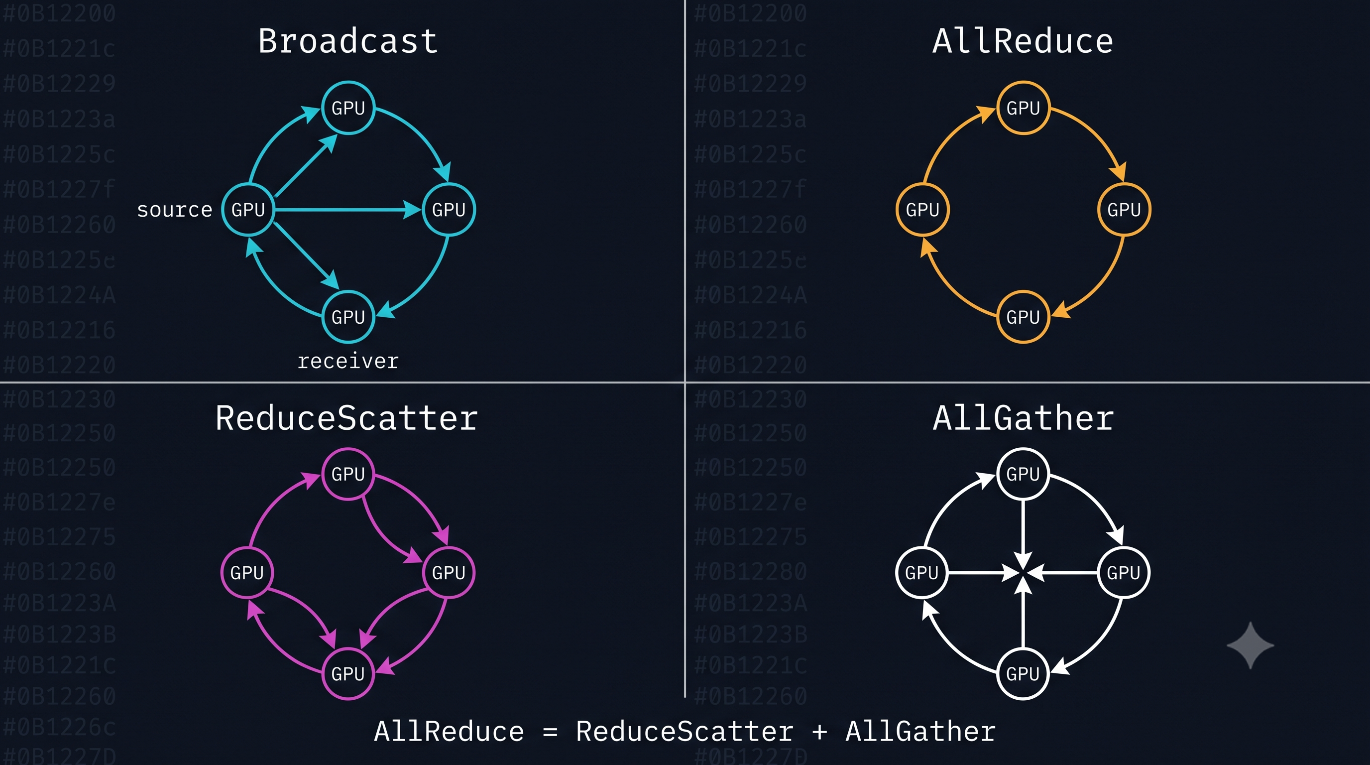
One rank owns a tensor; after the operation, every rank holds an identical copy.

Imagine rank 0 holds a weight tensor of shape [4096, 4096]. Data flows outward in a spanning tree: rank 0 sends to ranks 1 and 2, which each relay to two more, and so on. The source is singular; the destination is the entire communicator. Broadcast is most visible during model initialization (scattering initial weights from rank 0) and in pipeline parallelism stages where activations must be replicated across a tensor-parallel group.

AllReduce

Every rank contributes a tensor of equal shape; after the operation, every rank holds the element-wise reduction (typically summation) of all contributions.

This is the workhorse of data-parallel training. Rank 0 holds gradient shard G₀, rank 1 holds G₁, …, rank N-1 holds G_{N-1}. After AllReduce, every rank holds G₀ + G₁ + ... + G_{N-1}. No rank is privileged; the result is symmetric. The cost — when you fail to tune it — is the single largest bottleneck in large-scale training.

ReduceScatter

Every rank contributes a tensor; after the operation, rank i holds only the i-th chunk of the global reduction.

Think of it as a half-AllReduce. All N ranks hold full-sized tensors. They perform the reduction, but instead of broadcasting the result back to everyone, they distribute the chunks: rank 0 keeps the reduced first S/N elements, rank 1 keeps the next S/N, and so on. The output per rank is 1/N the size of the input. This asymmetry is the key insight exploited by FSDP and ZeRO.

AllGather

Every rank holds a shard of size S/N; after the operation, every rank holds the full concatenated tensor of size S.

This is the inverse of ReduceScatter. Rank i contributes its local shard, and the operation assembles all N shards into the complete tensor on every participant. In FSDP, this reconstructs the full parameter tensor on-demand before a forward or backward pass, then discards it immediately after — a temporal sharding strategy that minimizes peak memory.

2. AllReduce = ReduceScatter + AllGather: The Algebraic Identity That Powers FSDP

This is not a trick. It is a mathematically exact decomposition with profound engineering consequences.

The Identity

A ring AllReduce over N ranks on a tensor S is operationally identical to:

ReduceScatter: Each rank ends up with a reduced shard of size S/N
AllGather: Each rank broadcasts its shard so everyone reconstructs the full S

The intermediate state — where each rank holds only S/N bytes of fully-reduced data — is the key. The total bytes transferred across both phases equals that of a traditional AllReduce, but the decomposition exposes a seam that ZeRO-stage-3 and PyTorch FSDP exploit relentlessly.

Why FSDP Lives Here

Fully Sharded Data Parallel (FSDP), originally formalized through DeepSpeed ZeRO (Rajbhandari et al., 2019) and productionized in PyTorch, partitions model parameters, gradients, and optimizer states across ranks. The lifecycle of a parameter tensor looks like this:

Forward pass: AllGather reconstructs full weight tensor → compute → immediately free the gathered tensor
Backward pass: AllGather again for gradient computation → free → ReduceScatter accumulates and distributes gradient shards
Optimizer step: Each rank updates only its 1/N shard in-place

The ReduceScatter+AllGather decomposition is not just a theoretical nicety — it is the mechanism through which FSDP achieves near-linear memory scaling. A 70B parameter model that would require ~140 GB of GPU memory per rank in DDP now requires only 140/N GB in the steady-state sharded form. Megatron-LM’s throughput benchmarks (Narayanan et al., 2021) confirm that this decomposition, when paired with overlapped computation, sustains >50% Model FLOPs Utilization (MFU) on thousand-GPU runs — numbers that are impossible to reach with naive AllReduce.

3. Ring vs. Tree Algorithms: Deriving the Cost Model

The Ring Algorithm

In a ring AllReduce, N GPUs are arranged in a logical ring. The algorithm proceeds in two phases of N-1 steps each:

Phase 1 — ReduceScatter (N-1 steps): Each GPU sends S/N bytes to its neighbor and simultaneously receives S/N bytes, accumulating partial sums. After N-1 steps, each GPU holds one fully-reduced chunk.

Phase 2 — AllGather (N-1 steps): Each GPU forwards the chunk it just fully reduced, propagating it around the ring until every GPU holds all chunks.

Bandwidth Cost Derivation

In each of the 2(N-1) steps, each GPU sends and receives exactly S/N bytes. Total data sent per GPU:

Total bytes = 2(N-1) × S/N

Time to complete (assuming bidirectional bandwidth B per link, ignoring latency):

T_ring = 2(N-1)/N × S/B

As N → ∞, this converges to 2S/B — asymptotically bandwidth-optimal. This is the theoretical best any collective can achieve for AllReduce, because you cannot reduce the total bytes transferred below 2S (each element must leave and return to every rank). Ring AllReduce achieves this bound at scale, which is why NCCL defaults to it for large tensors on well-connected topologies (NCCL Developer Guide, 2023).

For small tensors, this derivation breaks down because latency dominates. Each step incurs a round-trip latency α, giving a corrected model:

T_ring = 2(N-1) × α + 2(N-1)/N × S/B

When S is small (kilobytes rather than megabytes), the 2(N-1)α term swamps the bandwidth term, and ring performs poorly at scale because latency multiplies with N.

Tree Algorithms

Tree-based collectives (binary tree, recursive halving-doubling) reduce the latency term to O(log N) steps at the cost of suboptimal bandwidth utilization — only (N-1)/N efficiency versus ring’s asymptotic optimality. NCCL’s TREE algorithm uses a virtual tree built on top of the physical NVLink/IB topology, trading per-step data volume for fewer synchronization points.

4. When NCCL Picks Ring vs. Tree: Threshold Logic and Topology Awareness

NCCL’s algorithm selection is not random. It is driven by a runtime heuristic that considers tensor size, inter-node topology, and the communicator’s rank geometry (NCCL GitHub source, src/graph/topo.cc).

Size threshold: For tensors below approximately 256 KB (the precise value is tunable), NCCL defaults to the TREE algorithm because latency — not bandwidth — is the bottleneck. Above 256 KB, ring’s bandwidth optimality wins. This threshold shifts upward in high-latency environments (e.g., RoCE over 100 GbE vs. NVLink).

Topology awareness: When NCCL detects NVSwitch fabric (e.g., DGX A100 or H100 nodes), intra-node communication is non-blocking at full bisection bandwidth. NCCL exploits this by fusing intra-node reduces before the inter-node ring step, effectively running a two-level hierarchy: a local AllReduce within the node using shared memory or NVLink, then a cross-node ring over InfiniBand. This is why NCCL_P2P_LEVEL and NCCL_SHM_DISABLE matter — they control whether NCCL uses NVLink peer-to-peer or falls back to PCIe, dramatically changing which algorithm wins.

Collnet: On clusters with InfiniBand in-network computing (SHARP acceleration), NCCL can offload AllReduce reduction to the switch fabric itself via the COLLNET algorithm, bypassing GPU memory bandwidth entirely for the reduction phase. This is exposed but only available on supported Mellanox/NVIDIA IB hardware.

5. The Tuning Knobs That Actually Move the Needle

`NCCL_ALGO`

Forces the algorithm selection: RING, TREE, COLLNET_DIRECT, COLLNET_CHAIN. Default is AUTO. In production, set to RING for large-model gradient syncs (tensors > 10 MB) and benchmark; switch to TREE only if you are latency-bound in a high-rank-count, small-tensor regime.

export NCCL_ALGO=RING

`NCCL_PROTO`

Controls the wire protocol. Three options with dramatically different characteristics:

Simple: Low overhead, high latency, largest chunk size. Best for saturating high-bandwidth NVLink on large tensors.
LL (Low Latency): Uses 8-byte data+flag pairs in a lock-step protocol. Halves effective bandwidth but cuts latency for small tensors. CPU polling instead of CUDA events.
LL128: 128-byte chunks with inline flags. The sweet spot — 7× the throughput of LL with nearly the same latency profile. Default for NVLink on modern hardware.

In practice: leave NCCL_PROTO=LL128 for NVLink intra-node and NCCL_PROTO=Simple for IB inter-node. Mixing protocols is valid per-communicator.

`NCCL_NTHREADS`

Controls the number of CUDA threads per NCCL block. Valid values: 64–512 (must be multiples of 64). Higher values increase throughput for large tensors by allowing wider SIMD-style reductions; lower values reduce occupancy pressure, leaving more SM resources for compute kernels that overlap with communication. For A100/H100 with CUDA graph-captured AllReduces, NCCL_NTHREADS=512 is generally optimal.

export NCCL_NTHREADS=512

`NCCL_NSOCKS_PERTHREAD`

Relevant only for socket-based transport (TCP/IP fallback when IB is absent). Controls parallelism within the socket transport layer. Default is 1; increasing to 4–8 can recover throughput on multi-GbE setups but is irrelevant on NVLink/IB. If you are seeing this knob matter in production, your topology is wrong — fix the IB fabric first.

6. Diagnosing a Slow AllReduce: `NCCL_DEBUG=INFO` and Nsight Systems

Slow AllReduce has three root causes: topology mismatch, protocol misconfiguration, and stragglers. The diagnostic workflow below isolates each in under 30 minutes.

Step 1: Enable NCCL Debug Logging

export NCCL_DEBUG=INFO
export NCCL_DEBUG_SUBSYS=ALL

On launch, NCCL will emit a topology detection report to stderr. The critical lines to examine:

NCCL INFO Trees [0] 1/-1/-1->0->-1 [1] 0/-1/-1->1->-1
NCCL INFO Channel 00/02 : 0 1 2 3 4 5 6 7
NCCL INFO Algorithm: Ring, Protocol: LL128

If you see NCCL INFO P2P no NVLink on a DGX system, something has disabled NVLink peer access — check nvidia-smi topo -m and NCCL_P2P_DISABLE. If Protocol: Simple appears where you expected LL128, check that NCCL_PROTO is not overridden downstream by a launcher script.

Also inspect the bandwidth report:

NCCL INFO NET/IB : Using [0]mlx5_0:1 [1]mlx5_1:1 ... SHARP off

SHARP off on a cluster that supports it means you are leaving in-network compute on the table. Contact your HPC admin.

Step 2: Profile with Nsight Systems

nsys profile \
  --trace=cuda,nvtx,nccl \
  --output=profile_%p \
  python train.py

Open the resulting .nsys-rep in the Nsight Systems GUI. Navigate to the NCCL row in the GPU timeline. You are looking for:

Gap analysis: Gaps between consecutive AllReduce kernels indicate compute-communication overlap failure. In a healthy FSDP run, AllGather for layer i+1 should overlap with the forward pass of layer i. If you see serialized sequences — AllGather → forward → AllGather → forward — your backward_prefetch and forward_prefetch policies in FSDP are not configured correctly.

Duration outliers: Sort AllReduce events by duration. A bimodal distribution (most fast, a few 10× slower) indicates a straggler rank. Cross-reference with NCCL_DEBUG output to find which rank is slow. Common causes: thermal throttling, PCIe contention from non-GPU processes, or asymmetric NVLink lane failures (check nvidia-smi nvlink --errorcounters).

Kernel fragmentation: If you see dozens of small AllReduce calls where you expected one, gradient bucketing is broken. In DDP, increase bucket_cap_mb from the default 25 MB to 200–500 MB. In FSDP, verify that limit_all_gathers=True is set to prevent unbounded AllGather fan-out.

Step 3: Bandwidth Sanity Check

Run NCCL’s built-in benchmark tool:

# From nccl-tests repository
./build/all_reduce_perf -b 8 -e 4G -f 2 -g 8

Compare the reported algbw (algorithm bandwidth) and busbw (bus bandwidth) against theoretical peak. On NVLink 4.0 (H100 SXM), busbw should reach ~900 GB/s intra-node. On 400 Gbps IB HDR200, inter-node busbw peaks near ~45 GB/s per GPU in an 8-GPU-per-node configuration. If you see less than 70% of theoretical, you have a transport or topology problem — not a training code problem.

Closing: The Mental Model That Unifies Everything

NCCL is not a black box. It is a bandwidth-optimal, topology-aware collective communication library whose behavior is almost entirely deterministic once you understand three things: which algorithm is selected, which protocol is used, and whether your physical topology matches NCCL’s logical model of it.

The ring AllReduce bound 2(N-1)/N × S/B is your ceiling. Every tuning decision — FSDP’s ReduceScatter+AllGather decomposition, protocol selection, thread count, overlap scheduling — is an attempt to approach that ceiling while keeping GPU compute utilization high. Narayanan et al. (2021) showed that Megatron-LM could sustain over 50% MFU at 1024-GPU scale precisely because they treated communication as a first-class engineering variable, not an afterthought. The same discipline, applied with the diagnostic tools above, is what separates a 35% MFU training run from a 55% one — a gap that, at thousand-GPU scale, represents millions of dollars in compute cost.

Master the primitives. Derive the costs. Instrument everything. The latency is always somewhere.

References

NVIDIA NCCL Developer Guide (2023). NCCL Operations and Algorithms. https://docs.nvidia.com/deeplearning/nccl/user-guide/docs/usage/operations.html
Narayanan, D., et al. (2021). Efficient Large-Scale Language Model Training on GPU Clusters Using Megatron-LM. SC ‘21. https://arxiv.org/abs/2104.04473
Rajbhandari, S., et al. (2019). ZeRO: Memory Optimizations Toward Training Trillion Parameter Models. https://arxiv.org/abs/1910.02054
NCCL GitHub Repository. src/graph/topo.cc, src/enqueue.cc. https://github.com/NVIDIA/nccl
PyTorch FSDP Documentation. Fully Sharded Data Parallel. https://pytorch.org/docs/stable/fsdp.html

BibTeX

@article{fp4-2606009,
  title   = {NCCL Collective Operations: The Architecture of Distributed Gradient Truth},
  author  = {fp4 editorial desk},
  year    = {2026},
  url     = {https://fp4.dev/system/nccl-collective-operations/},
  journal = {fp4}
}